Shapes

This section presents an overview of the shape plugins that are released along with the renderer.

In Mitsuba 2, shapes define surfaces that mark transitions between different types of materials. For instance, a shape could describe a boundary between air and a solid object, such as a piece of rock. Alternatively, a shape can mark the beginning of a region of space that isn’t solid at all, but rather contains a participating medium, such as smoke or steam. Finally, a shape can be used to create an object that emits light on its own.

Shapes are usually declared along with a surface scattering model named BSDF (see the respective section). This BSDF characterizes what happens at the surface. In the XML scene description language, this might look like the following:

<scene version=2.0.0>
    <shape type=".. shape type ..">
        .. shape parameters ..

        <bsdf type=".. BSDF type ..">
            .. bsdf parameters ..
        </bsdf>

        <!-- Alternatively: reference a named BSDF that
             has been declared previously

             <ref id="my_bsdf"/>
        -->
    </shape>
</scene>

The following subsections discuss the available shape types in greater detail.

Wavefront OBJ mesh loader (obj)

Parameter	Type	Description
filename	string	Filename of the OBJ file that should be loaded
face_normals	boolean	When set to true, any existing or computed vertex normals are discarded and face normals will instead be used during rendering. This gives the rendered object a faceted appearance. (Default: false)
flip_tex_coords	boolean	Treat the vertical component of the texture as inverted? Most OBJ files use this convention. (Default: true)
to_world	transform	Specifies an optional linear object-to-world transformation. (Default: none, i.e. object space = world space)

This plugin implements a simple loader for Wavefront OBJ files. It handles meshes containing triangles and quadrilaterals, and it also imports vertex normals and texture coordinates.

Loading an ordinary OBJ file is as simple as writing:

<shape type="obj">
    <string name="filename" value="my_shape.obj"/>
</shape>

Note

Importing geometry via OBJ files should only be used as an absolutely last resort. Due to inherent limitations of this format, the files tend to be unreasonably large, and parsing them requires significant amounts of memory and processing power. What’s worse is that the internally stored data is often truncated, causing a loss of precision. If possible, use the ply or serialized plugins instead.

PLY (Stanford Triangle Format) mesh loader (ply)

Parameter	Type	Description
filename	string	Filename of the PLY file that should be loaded
face_normals	boolean	When set to true, any existing or computed vertex normals are discarded and face normals will instead be used during rendering. This gives the rendered object a faceted appearance. (Default: false)
to_world	transform	Specifies an optional linear object-to-world transformation. (Default: none, i.e. object space = world space)

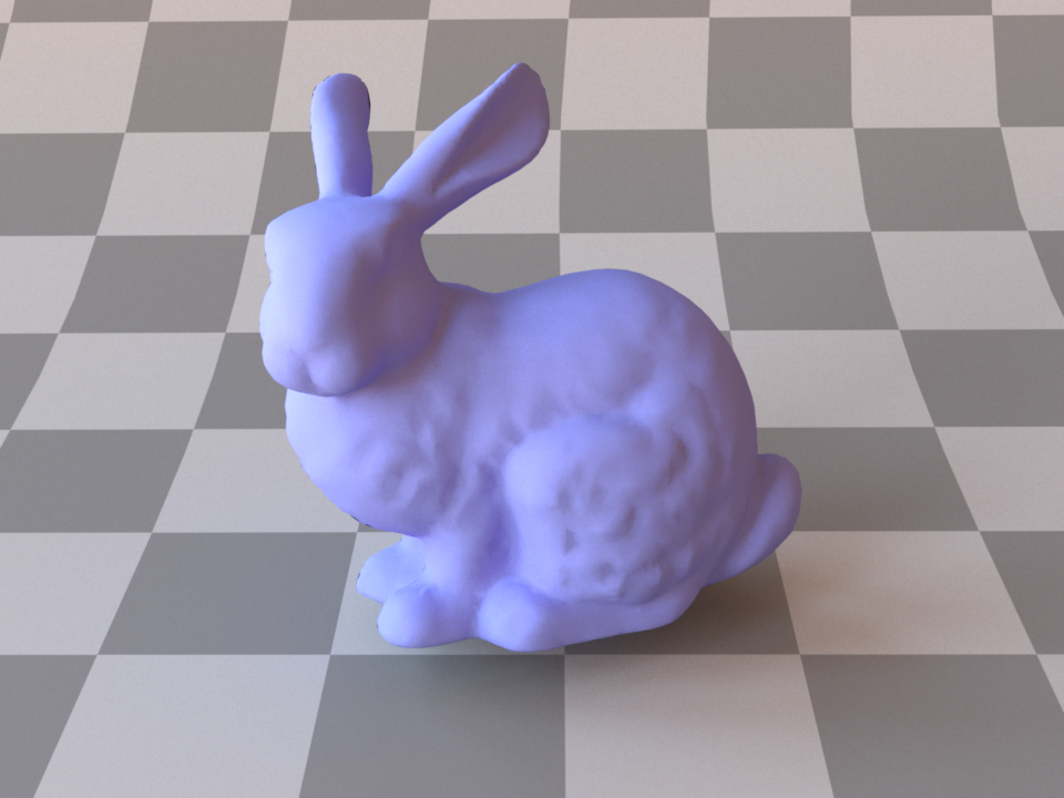
The Stanford bunny loaded with face_normals=false.

The Stanford bunny loaded with face_normals=true. Note the faceted appearance.

This plugin implements a fast loader for the Stanford PLY format (both the ASCII and binary format, which is preferred for performance reasons). The current plugin implementation supports triangle meshes with optional UV coordinates, vertex normals and other custom vertex or face attributes.

Consecutive attributes with names sharing a common prefix and using one of the following schemes:

{prefix}_{x|y|z|w}, {prefix}_{r|g|b|a}, {prefix}_{0|1|2|3}, {prefix}_{1|2|3|4}

will be group together under a single multidimentional attribute named {vertex|face}_{prefix}.

RGB color attributes can also be defined without a prefix, following the naming scheme {r|g|b|a} or {red|green|blue|alpha}. Those attributes will be group together under a single multidimentional attribute named {vertex|face}_color.

Note

Values stored in a RBG color attribute will automatically be converted into spectal model coefficients when using a spectral variant of the renderer.

Serialized mesh loader (serialized)

Parameter	Type	Description
filename	string	Filename of the OBJ file that should be loaded
shape_index	integer	A .serialized file may contain several separate meshes. This parameter specifies which one should be loaded. (Default: 0, i.e. the first one)
face_normals	boolean	When set to true, any existing or computed vertex normals are discarded and emph{face normals} will instead be used during rendering. This gives the rendered object a faceted appearance.(Default: false)
to_world	transform	Specifies an optional linear object-to-world transformation. (Default: none, i.e. object space = world space)

The serialized mesh format represents the most space and time-efficient way of getting geometry information into Mitsuba 2. It stores indexed triangle meshes in a lossless gzip-based encoding that (after decompression) nicely matches up with the internally used data structures. Loading such files is considerably faster than the ply plugin and orders of magnitude faster than the obj plugin.

Format description

The serialized file format uses the little endian encoding, hence all fields below should be interpreted accordingly. The contents are structured as follows:

Type	Content
uint16	File format identifier: 0x041C
uint16	File version identifier. Currently set to 0x0004
\(\rightarrow\)	From this point on, the stream is compressed by the DEFLATE algorithm.
\(\rightarrow\)	The used encoding is that of the zlib library.
uint32	An 32-bit integer whose bits can be used to specify the following flags: 0x0001: The mesh data includes per-vertex normals 0x0002: The mesh data includes texture coordinates 0x0008: The mesh data includes vertex colors 0x0010: Use face normals instead of smothly interpolated vertex normals. Equivalent to specifying face_normals=true to the plugin. 0x1000: The subsequent content is represented in single precision 0x2000: The subsequent content is represented in double precision
string	A null-terminated string (utf-8), which denotes the name of the shape.
uint64	Number of vertices in the mesh
uint64	Number of triangles in the mesh
array	Array of all vertex positions (X, Y, Z, X, Y, Z, …) specified in binary single or double precision format (as denoted by the flags)
array	Array of all vertex normal directions (X, Y, Z, X, Y, Z, …) specified in binary single or double precision format. When the mesh has no vertex normals, this field is omitted.
array	Array of all vertex texture coordinates (U, V, U, V, …) specified in binary single or double precision format. When the mesh has no texture coordinates, this field is omitted.
array	Array of all vertex colors (R, G, B, R, G, B, …) specified in binary single or double precision format. When the mesh has no vertex colors, this field is omitted.
array	Indexed triangle data ([i1, i2, i3], [i1, i2, i3], ..) specified in uint32 or in uint64 format (the latter is used when the number of vertices exceeds 0xFFFFFFFF).

Multiple shapes

It is possible to store multiple meshes in a single .serialized file. This is done by simply concatenating their data streams, where every one is structured according to the above description. Hence, after each mesh, the stream briefly reverts back to an uncompressed format, followed by an uncompressed header, and so on. This is neccessary for efficient read access to arbitrary sub-meshes.

End-of-file dictionary

In addition to the previous table, a .serialized file also concludes with a brief summary at the end of the file, which specifies the starting position of each sub-mesh:

Type	Content
uint64	File offset of the first mesh (in bytes)—this is always zero.
uint64	File offset of the second mesh
\(\cdots\)	\(\cdots\)
uint64	File offset of the last sub-shape
uint32	Total number of meshes in the .serialized file

Sphere (sphere)

Parameter	Type	Description
center	point	Center of the sphere (Default: (0, 0, 0))
radius	float	Radius of the sphere (Default: 1)
flip_normals	boolean	Is the sphere inverted, i.e. should the normal vectors be flipped? (Default:false, i.e. the normals point outside)
to_world	transform	Specifies an optional linear object-to-world transformation. Note that non-uniform scales and shears are not permitted! (Default: none, i.e. object space = world space)

Basic example

A textured sphere with the default parameterization

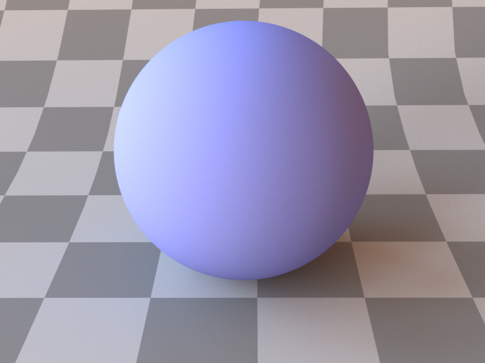
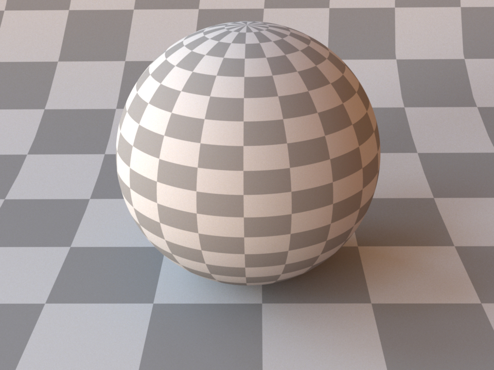
This shape plugin describes a simple sphere intersection primitive. It should always be preferred over sphere approximations modeled using triangles.

A sphere can either be configured using a linear to_world transformation or the center and radius parameters (or both). The two declarations below are equivalent.

<shape type="sphere">
    <transform name="to_world">
        <scale value="2"/>
        <translate x="1" y="0" z="0"/>
    </transform>
    <bsdf type="diffuse"/>
</shape>

<shape type="sphere">
    <point name="center" x="1" y="0" z="0"/>
    <float name="radius" value="2"/>
    <bsdf type="diffuse"/>
</shape>

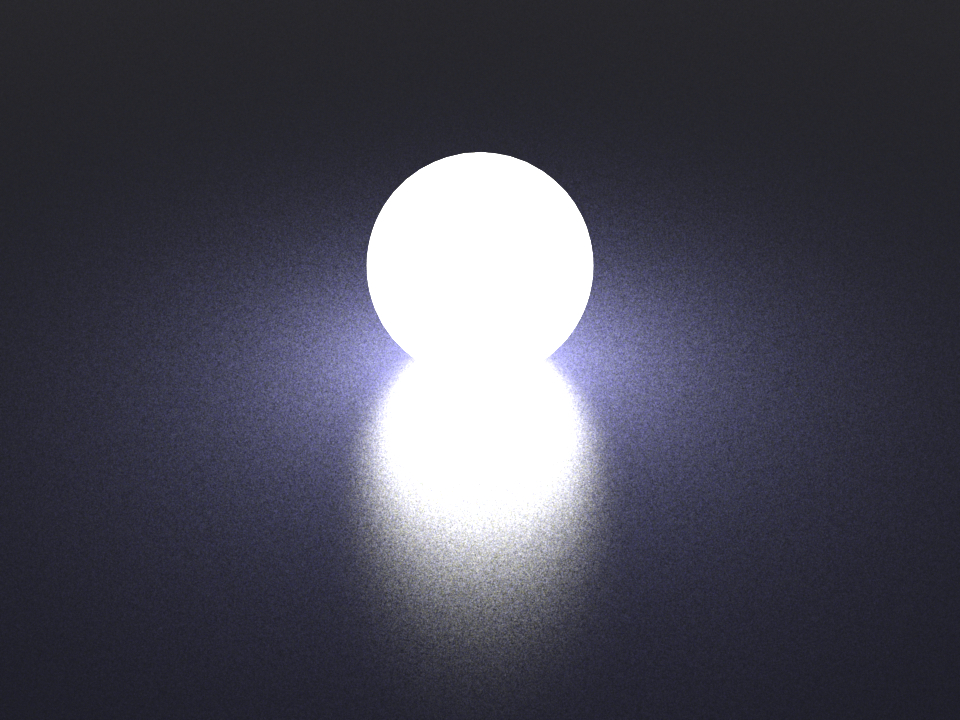
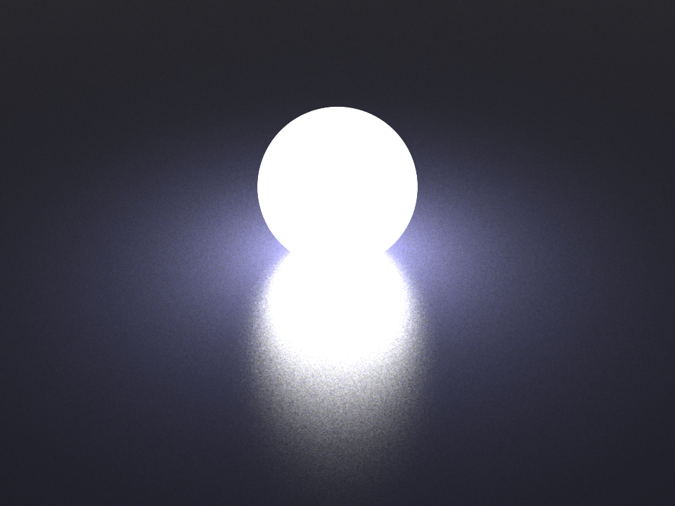
When a sphere shape is turned into an area light source, Mitsuba 2 switches to an efficient sampling strategy by Fred Akalin that has particularly low variance. This makes it a good default choice for lighting new scenes.

Spherical area light modeled using triangles

Spherical area light modeled using the sphere plugin

Cylinder (cylinder)

Parameter	Type	Description
p0	point	Object-space starting point of the cylinder’s centerline. (Default: (0, 0, 0))
p1	point	Object-space endpoint of the cylinder’s centerline (Default: (0, 0, 1))
radius	float	Radius of the cylinder in object-space units (Default: 1)
flip_normals	boolean	Is the cylinder inverted, i.e. should the normal vectors be flipped? (Default: false, i.e. the normals point outside)
to_world	transform	Specifies an optional linear object-to-world transformation. Note that non-uniform scales are not permitted! (Default: none, i.e. object space = world space)

Cylinder with the default one-sided shading

Cylinder with two-sided shading

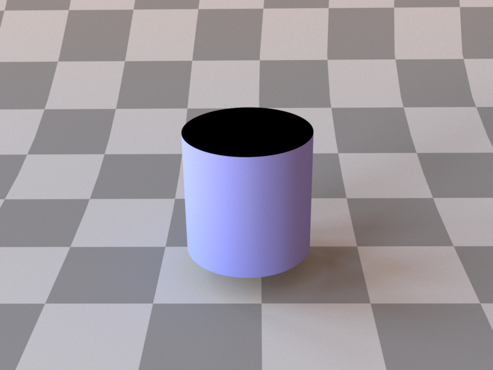
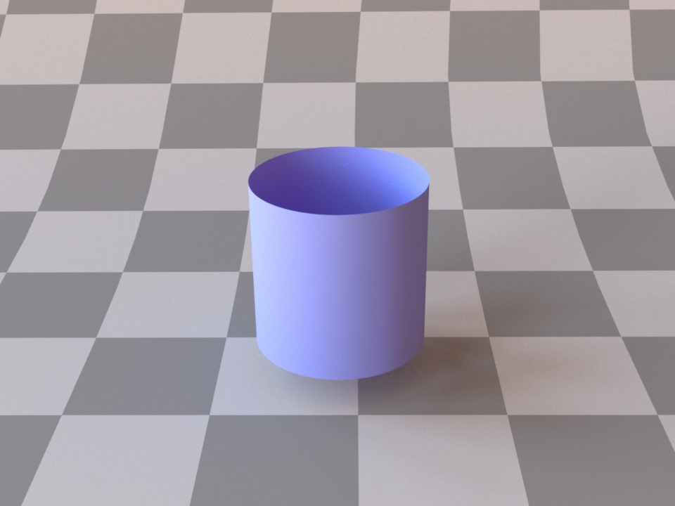
This shape plugin describes a simple cylinder intersection primitive. It should always be preferred over approximations modeled using triangles. Note that the cylinder does not have endcaps – also, its normals point outward, which means that the inside will be treated as fully absorbing by most material models. If this is not desirable, consider using the twosided plugin.

A simple example for instantiating a cylinder, whose interior is visible:

<shape type="cylinder">
    <float name="radius" value="0.3"/>
    <bsdf type="twosided">
        <bsdf type="diffuse"/>
    </bsdf>
</shape>

Cone (cone)

Parameter	Type	Description
p0	point	Object-space starting point of the cone’s centerline. (Base) (Default: (0, 0, 0))
p1	point	Object-space endpoint of the cone’s centerline (Default: (0, 0, 1)) (Tip)
radius	float	Radius of the cone in object-space units (Default: 1)
flip_normals	boolean	Is the cone inverted, i.e. should the normal vectors be flipped? (Default: false, i.e. the normals point outside)
to_world	transform	Specifies an optional linear object-to-world transformation. Note that non-uniform scales are not permitted! (Default: none, i.e. object space = world space)

Cone with the default configuration and diffuse BSDF

Upside down cone with two-sided shading

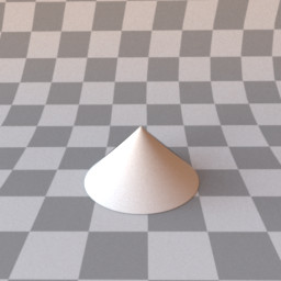
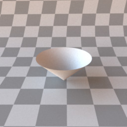
This shape plugin describes a simple cone intersection primitive. It should always be preferred over approximations modeled using triangles. Note that the cone does not have endcaps – also, its normals point outward, which means that the inside will be treated as fully absorbing by most material models. If this is not desirable, consider using the twosided plugin.

A simple example for instantiating a cone, whose interior is visible:

<shape type="cone">
    <float name="radius" value="0.3"/>
    <bsdf type="twosided">
        <bsdf type="diffuse"/>
    </bsdf>
</shape>

Disk (disk)

Parameter	Type	Description
flip_normals	boolean	Is the disk inverted, i.e. should the normal vectors be flipped? (Default: false)
to_world	transform	Specifies a linear object-to-world transformation. Note that non-uniform scales are not permitted! (Default: none, i.e. object space = world space)

Basic example

A textured disk with the default parameterization

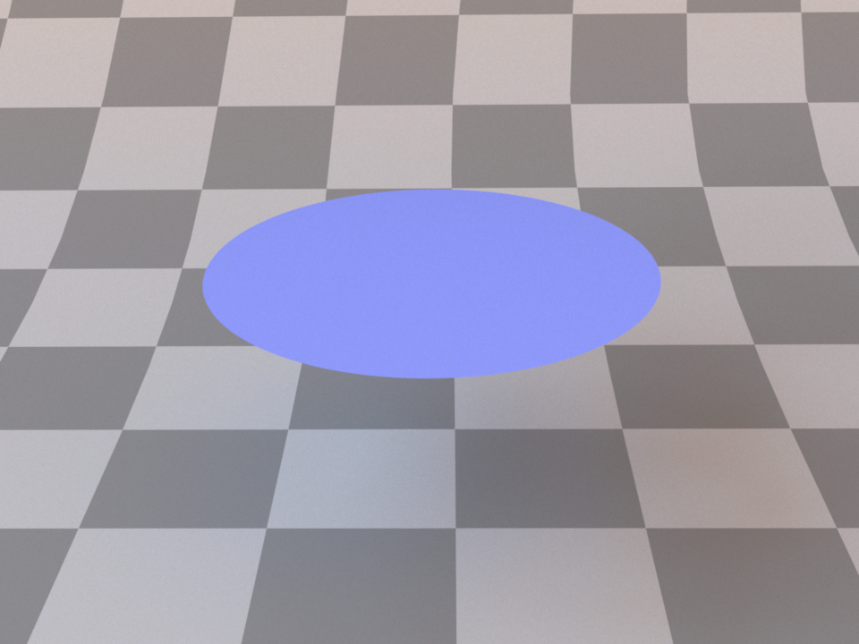
This shape plugin describes a simple disk intersection primitive. It is usually preferable over discrete approximations made from triangles.

By default, the disk has unit radius and is located at the origin. Its surface normal points into the positive Z-direction. To change the disk scale, rotation, or translation, use the to_world parameter.

The following XML snippet instantiates an example of a textured disk shape:

<shape type="disk">
    <bsdf type="diffuse">
        <texture name="reflectance" type="checkerboard">
            <transform name="to_uv">
                <scale x="2" y="10" />
            </transform>
        </texture>
    </bsdf>
</shape>

Rectangle (rectangle)

Parameter	Type	Description
flip_normals	boolean	Is the rectangle inverted, i.e. should the normal vectors be flipped? (Default: false)
to_world	transform	Specifies a linear object-to-world transformation. (Default: none (i.e. object space = world space))

Basic example

A textured rectangle with the default parameterization

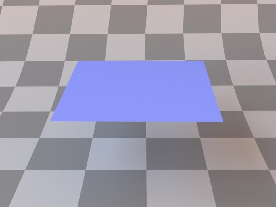
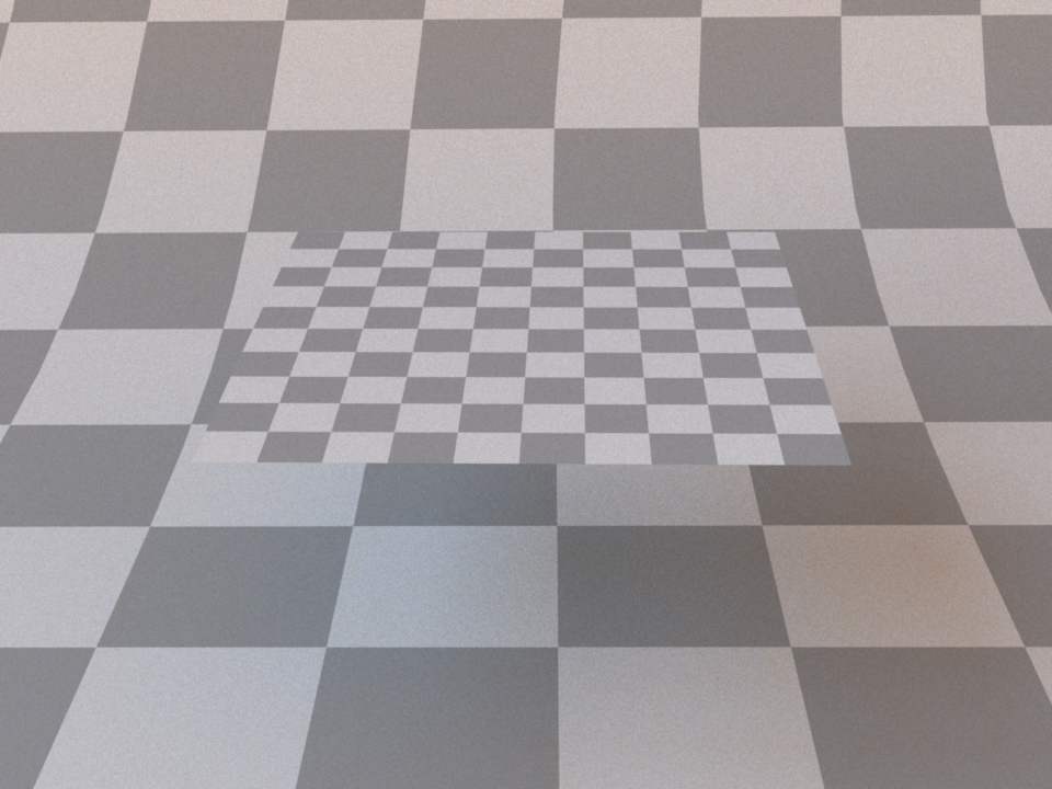
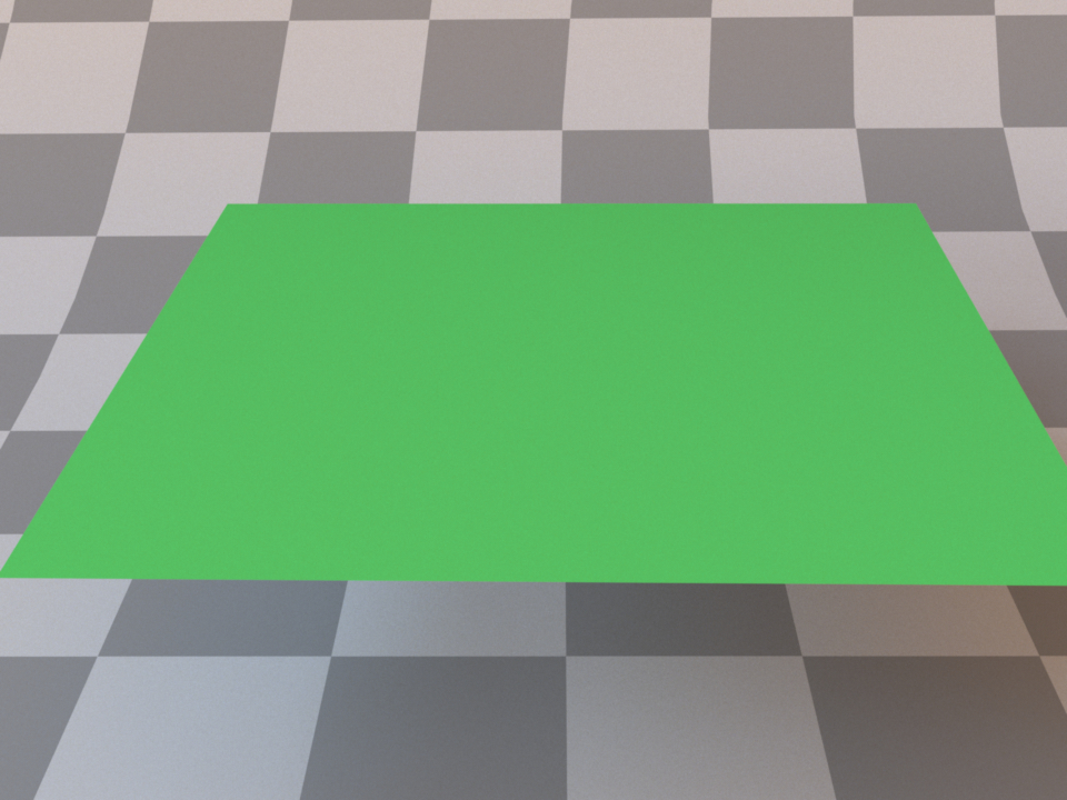
This shape plugin describes a simple rectangular shape primitive. It is mainly provided as a convenience for those cases when creating and loading an external mesh with two triangles is simply too tedious, e.g. when an area light source or a simple ground plane are needed. By default, the rectangle covers the XY-range \([-1,1]\times[-1,1]\) and has a surface normal that points into the positive Z-direction. To change the rectangle scale, rotation, or translation, use the to_world parameter.

The following XML snippet showcases a simple example of a textured rectangle:

<shape type="rectangle">
    <bsdf type="diffuse">
        <texture name="reflectance" type="checkerboard">
            <transform name="to_uv">
                <scale x="5" y="5" />
            </transform>
        </texture>
    </bsdf>
</shape>

Cube (cube)

Parameter	Type	Description
to_world	transform	Specifies an optional linear object-to-world transformation. (Default: none (i.e. object space = world space))

This shape plugin describes a cube intersection primitive, based on the triangle mesh class.

Shape group (shapegroup)

Parameter	Type	Description
(Nested plugin)	shape	One or more shapes that should be made available for geometry instancing

This plugin implements a container for shapes that should be made available for geometry instancing. Any shapes placed in a shapegroup will not be visible on their own—instead, the renderer will precompute ray intersection acceleration data structures so that they can efficiently be referenced many times using the Instance (instance) plugin. This is useful for rendering things like forests, where only a few distinct types of trees have to be kept in memory. An example is given below:

<!-- Declare a named shape group containing two objects -->
<shape type="shapegroup" id="my_shape_group">
    <shape type="ply">
        <string name="filename" value="data.ply"/>
        <bsdf type="roughconductor"/>
    </shape>
    <shape type="sphere">
        <transform name="to_world">
            <scale value="5"/>
            <translate y="20"/>
        </transform>
        <bsdf type="diffuse"/>
    </shape>
</shape>

<!-- Instantiate the shape group without any kind of transformation -->
<shape type="instance">
    <ref id="my_shape_group"/>
</shape>

<!-- Create instance of the shape group, but rotated, scaled, and translated -->
<shape type="instance">
    <ref id="my_shape_group"/>
    <transform name="to_world">
        <rotate x="1" angle="45"/>
        <scale value="1.5"/>
        <translate z="10"/>
    </transform>
</shape>

Instance (instance)

Parameter	Type	Description
(Nested plugin)	shapegroup	A reference to a shape group that should be instantiated.
to_world	transform	Specifies a linear object-to-world transformation. (Default: none (i.e. object space = world space))

This plugin implements a geometry instance used to efficiently replicate geometry many times. For details on how to create instances, refer to the Shape group (shapegroup) plugin.

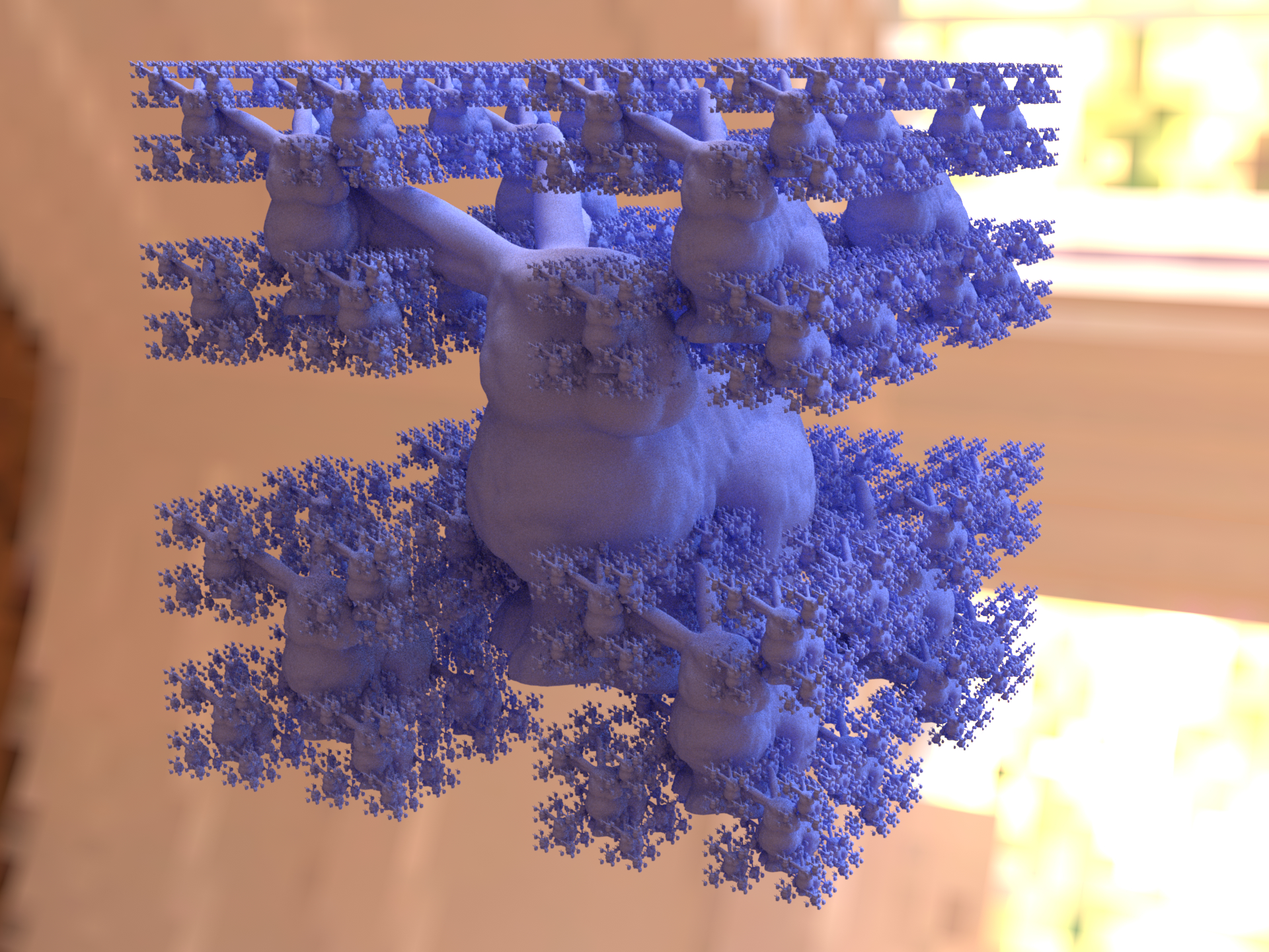
The Stanford bunny loaded a single time and instantiated 1365 times (equivalent to 100 million triangles)

Warning

• Note that it is not possible to assign a different material to each instance — the material assignment specified within the shape group is the one that matters.

• Shape groups cannot be used to replicate shapes with attached emitters, sensors, or subsurface scattering models.

BSDFs

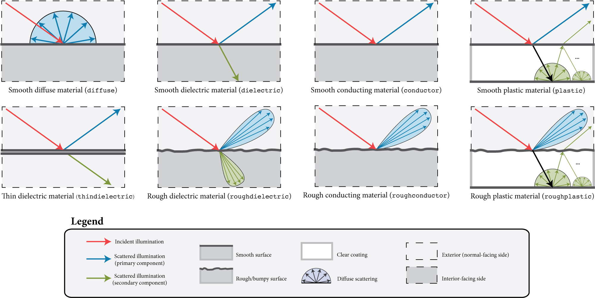
Schematic overview of the most important surface scattering models in Mitsuba 2. The arrows indicate possible outcomes of an interaction with a surface that has the respective model applied to it.

Surface scattering models describe the manner in which light interacts with surfaces in the scene. They conveniently summarize the mesoscopic scattering processes that take place within the material and cause it to look the way it does. This represents one central component of the material system in Mitsuba 2—another part of the renderer concerns itself with what happens in between surface interactions. For more information on this aspect, please refer to the sections regarding participating media. This section presents an overview of all surface scattering models that are supported, along with their parameters.

To achieve realistic results, Mitsuba 2 comes with a library of general-purpose surface scattering models such as glass, metal, or plastic. Some model plugins can also act as modifiers that are applied on top of one or more scattering models.

Throughout the documentation and within the scene description language, the word BSDF is used synonymously with the term surface scattering model. This is an abbreviation for Bidirectional Scattering Distribution Function, a more precise technical term.

In Mitsuba 2, BSDFs are assigned to shapes, which describe the visible surfaces in the scene. In the scene description language, this assignment can either be performed by nesting BSDFs within shapes, or they can be named and then later referenced by their name. The following fragment shows an example of both kinds of usages:

<scene version=2.0.0>
    <!-- Creating a named BSDF for later use -->
    <bsdf type=".. BSDF type .." id="my_named_material">
        <!-- BSDF parameters go here -->
    </bsdf>

    <shape type="sphere">
        <!-- Example of referencing a named material -->
        <ref id="my_named_material"/>
    </shape>

    <shape type="sphere">
        <!-- Example of instantiating an unnamed material -->
        <bsdf type=".. BSDF type ..">
            <!-- BSDF parameters go here -->
        </bsdf>
    </shape>
</scene>

It is generally more economical to use named BSDFs when they are used in several places, since this reduces the internal memory usage.

Correctness considerations

A vital consideration when modeling a scene in a physically-based rendering system is that the used materials do not violate physical properties, and that their arrangement is meaningful. For instance, imagine having designed an architectural interior scene that looks good except for a white desk that seems a bit too dark. A closer inspection reveals that it uses a Lambertian material with a diffuse reflectance of 0.9.

In many rendering systems, it would be feasible to increase the reflectance value above 1.0 in such a situation. But in Mitsuba, even a small surface that reflects a little more light than it receives will likely break the available rendering algorithms, or cause them to produce otherwise unpredictable results. In fact, the right solution in this case would be to switch to a different the lighting setup that causes more illumination to be received by the desk and then reduce the material’s reflectance—after all, it is quite unlikely that one could find a real-world desk that reflects 90% of all incident light.

As another example of the necessity for a meaningful material description, consider the glass model illustrated in the figure below. Here, careful thinking is needed to decompose the object into boundaries that mark index of refraction-changes. If this is done incorrectly and a beam of light can potentially pass through a sequence of incompatible index of refraction changes (e.g. 1.00 to 1.33 followed by 1.50 to 1.33), the output is undefined and will quite likely even contain inaccuracies in parts of the scene that are far away from the glass.

Some of the scattering models in Mitsuba need to know the indices of refraction on the exterior and interior-facing side of a surface. It is therefore important to decompose the mesh into meaningful separate surfaces corresponding to each index of refraction change. The example here shows such a decomposition for a water-filled Glass.

Smooth diffuse material (diffuse)

Parameter	Type	Description
reflectance	spectrum or texture	Specifies the diffuse albedo of the material (Default: 0.5)

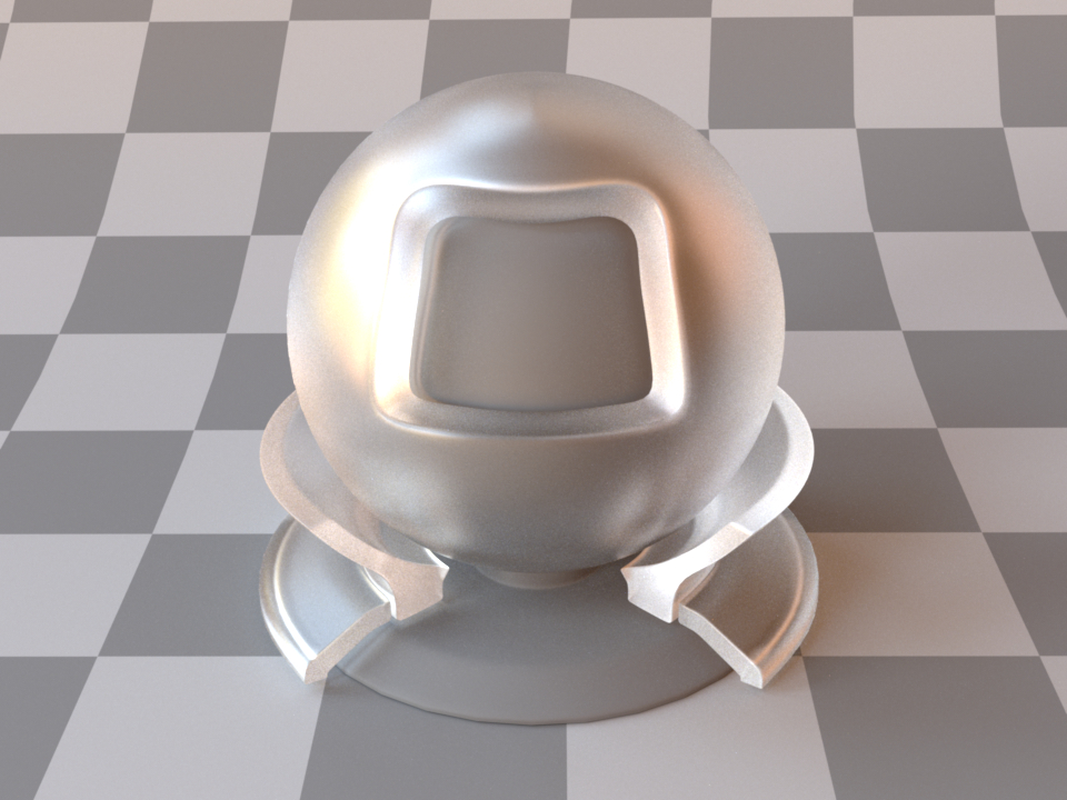
The smooth diffuse material (also referred to as Lambertian) represents an ideally diffuse material with a user-specified amount of reflectance. Any received illumination is scattered so that the surface looks the same independently of the direction of observation.

Homogeneous reflectance

Textured reflectance

Apart from a homogeneous reflectance value, the plugin can also accept a nested or referenced texture map to be used as the source of reflectance information, which is then mapped onto the shape based on its UV parameterization. When no parameters are specified, the model uses the default of 50% reflectance.

Note that this material is one-sided—that is, observed from the back side, it will be completely black. If this is undesirable, consider using the twosided BRDF adapter plugin. The following XML snippet describes a diffuse material, whose reflectance is specified as an sRGB color:

<bsdf type="diffuse">
    <rgb name="reflectance" value="0.2, 0.25, 0.7"/>
</bsdf>

Alternatively, the reflectance can be textured:

<bsdf type="diffuse">
    <texture type="bitmap" name="reflectance">
        <string name="filename" value="wood.jpg"/>
    </texture>
</bsdf>

Smooth dielectric material (dielectric)

Parameter	Type	Description
int_ior	float or string	Interior index of refraction specified numerically or using a known material name. (Default: bk7 / 1.5046)
ext_ior	float or string	Exterior index of refraction specified numerically or using a known material name. (Default: air / 1.000277)
specular_reflectance	spectrum or texture	Optional factor that can be used to modulate the specular reflection component. Note that for physical realism, this parameter should never be touched. (Default: 1.0)
specular_transmittance	spectrum or texture	Optional factor that can be used to modulate the specular transmission component. Note that for physical realism, this parameter should never be touched. (Default: 1.0)

Air ↔ Water (IOR: 1.33) interface.

Air ↔ Diamond (IOR: 2.419)

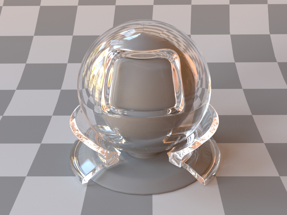
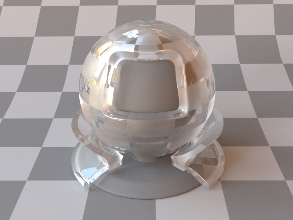
This plugin models an interface between two dielectric materials having mismatched indices of refraction (for instance, water ↔ air). Exterior and interior IOR values can be specified independently, where “exterior” refers to the side that contains the surface normal. When no parameters are given, the plugin activates the defaults, which describe a borosilicate glass (BK7) ↔ air interface.

In this model, the microscopic structure of the surface is assumed to be perfectly smooth, resulting in a degenerate BSDF described by a Dirac delta distribution. This means that for any given incoming ray of light, the model always scatters into a discrete set of directions, as opposed to a continuum. For a similar model that instead describes a rough surface microstructure, take a look at the roughdielectric plugin.

This snippet describes a simple air-to-water interface

<shape type="...">
    <bsdf type="dielectric">
        <string name="int_ior" value="water"/>
        <string name="ext_ior" value="air"/>
    </bsdf>
<shape>

When using this model, it is crucial that the scene contains meaningful and mutually compatible indices of refraction changes—see the section about correctness considerations for a description of what this entails.

In many cases, we will want to additionally describe the medium within a dielectric material. This requires the use of a rendering technique that is aware of media (e.g. the volumetric path tracer). An example of how one might describe a slightly absorbing piece of glass is shown below:

<shape type="...">
    <bsdf type="dielectric">
        <float name="int_ior" value="1.504"/>
        <float name="ext_ior" value="1.0"/>
    </bsdf>

    <medium type="homogeneous" name="interior">
        <float name="scale" value="4"/>
        <rgb name="sigma_t" value="1, 1, 0.5"/>
        <rgb name="albedo" value="0.0, 0.0, 0.0"/>
    </medium>
<shape>

In polarized rendering modes, the material automatically switches to a polarized implementation of the underlying Fresnel equations that quantify the reflectance and transmission.

Note

Dispersion is currently unsupported but will be enabled in a future release.

Instead of specifying numerical values for the indices of refraction, Mitsuba 2 comes with a list of presets that can be specified with the material parameter:

Name	Value	Name	Value
vacuum	1.0	acetone	1.36
bromine	1.661	bk7	1.5046
helium	1.00004	ethanol	1.361
water ice	1.31	sodium chloride	1.544
hydrogen	1.00013	carbon tetrachloride	1.461
fused quartz	1.458	amber	1.55
air	1.00028	glycerol	1.4729
pyrex	1.470	pet	1.575
carbon dioxide	1.00045	benzene	1.501
acrylic glass	1.49	diamond	2.419
water	1.3330	silicone oil	1.52045
polypropylene	1.49

This table lists all supported material names along with along with their associated index of refraction at standard conditions. These material names can be used with the plugins dielectric, roughdielectric, plastic , as well as roughplastic.

Thin dielectric material (thindielectric)

Parameter	Type	Description
int_ior	float or string	Interior index of refraction specified numerically or using a known material name. (Default: bk7 / 1.5046)
ext_ior	float or string	Exterior index of refraction specified numerically or using a known material name. (Default: air / 1.000277)
specular_reflectance	spectrum or texture	Optional factor that can be used to modulate the specular reflection component. Note that for physical realism, this parameter should never be touched. (Default: 1.0)
specular_transmittance	spectrum or texture	Optional factor that can be used to modulate the specular transmission component. Note that for physical realism, this parameter should never be touched. (Default: 1.0)

Dielectric

Thindielectric

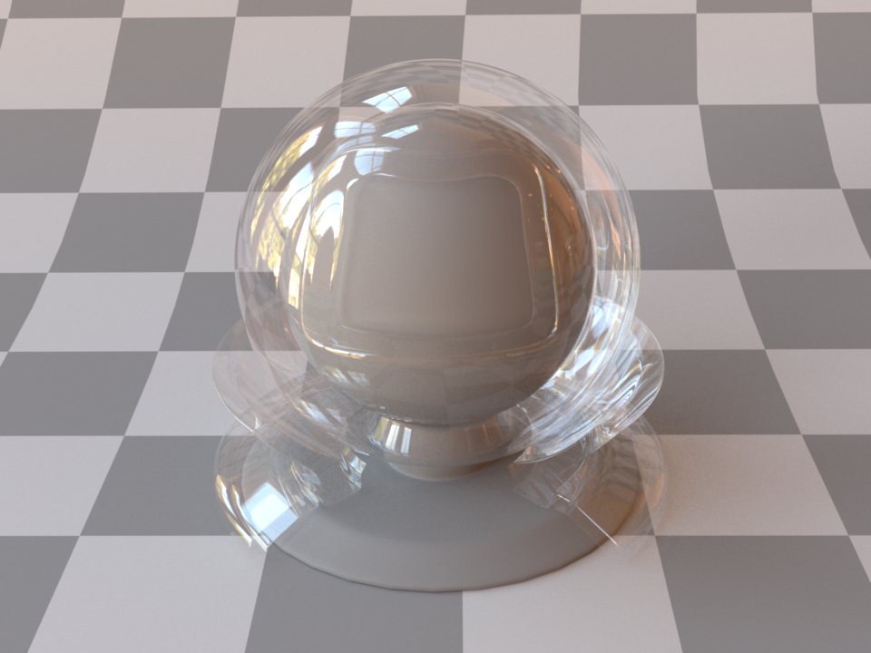
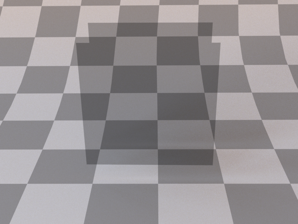
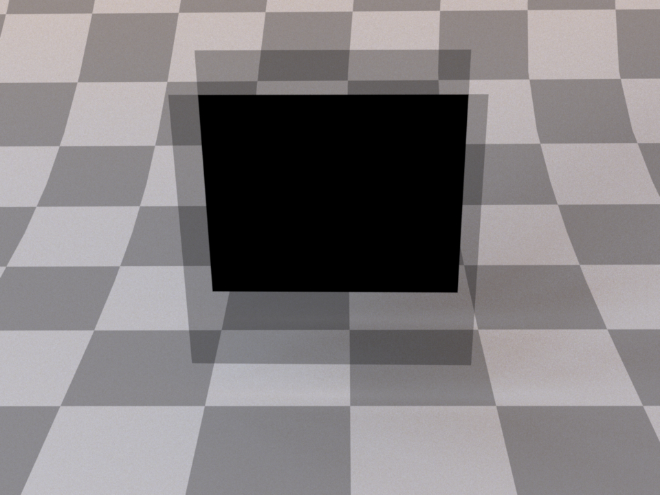
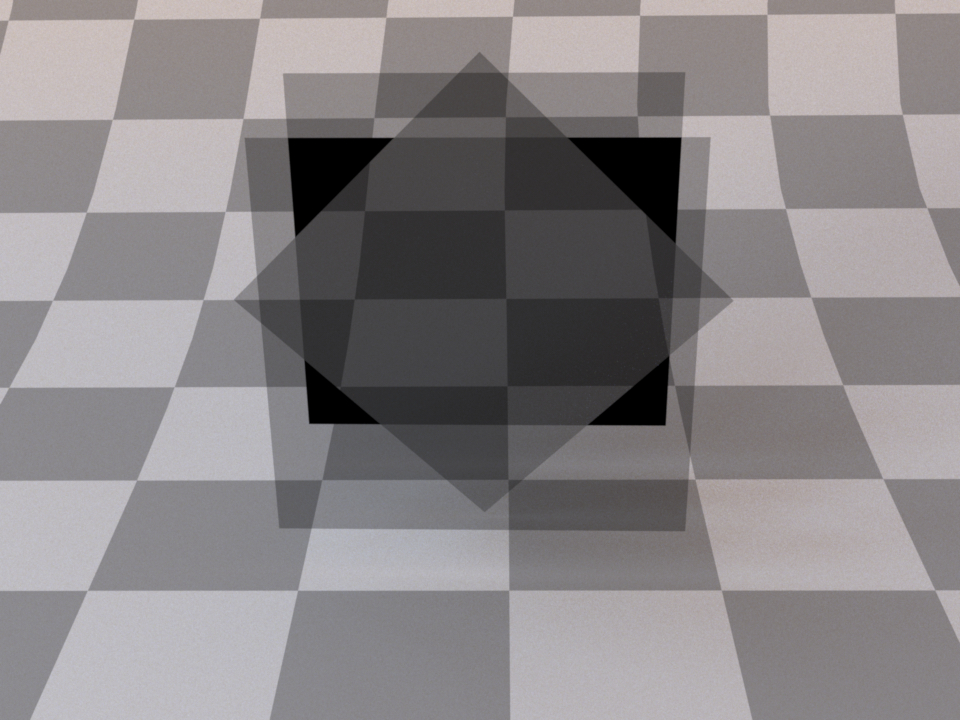
This plugin models a thin dielectric material that is embedded inside another dielectric—for instance, glass surrounded by air. The interior of the material is assumed to be so thin that its effect on transmitted rays is negligible, Hence, light exits such a material without any form of angular deflection (though there is still specular reflection). This model should be used for things like glass windows that were modeled using only a single sheet of triangles or quads. On the other hand, when the window consists of proper closed geometry, dielectric is the right choice. This is illustrated below:

The dielectric plugin models a single transition from one index of refraction to another

The thindielectric plugin models a pair of interfaces causing a transient index of refraction change

The implementation correctly accounts for multiple internal reflections inside the thin dielectric at no significant extra cost, i.e. paths of the type \(R, TRT, TR^3T, ..\) for reflection and \(TT, TR^2, TR^4T, ..\) for refraction, where \(T\) and \(R\) denote individual reflection and refraction events, respectively.

Similar to the dielectric plugin, IOR values can either be specified numerically, or based on a list of known materials (see the corresponding table in the dielectric reference). When no parameters are given, the plugin activates the default settings, which describe a borosilicate glass (BK7) ↔ air interface.

Rough dielectric material (roughdielectric)

Parameter	Type	Description
int_ior	float or string	Interior index of refraction specified numerically or using a known material name. (Default: bk7 / 1.5046)
ext_ior	float or string	Exterior index of refraction specified numerically or using a known material name. (Default: air / 1.000277)
specular_reflectance, specular_transmittance	spectrum or texture	Optional factor that can be used to modulate the specular reflection/transmission components. Note that for physical realism, these parameters should never be touched. (Default: 1.0)
distribution	string	Specifies the type of microfacet normal distribution used to model the surface roughness. beckmann: Physically-based distribution derived from Gaussian random surfaces. This is the default. ggx: The GGX [WMLT07] distribution (also known as Trowbridge-Reitz [TR75] distribution) was designed to better approximate the long tails observed in measurements of ground surfaces, which are not modeled by the Beckmann distribution.
alpha, alpha_u, alpha_v	texture or float	Specifies the roughness of the unresolved surface micro-geometry along the tangent and bitangent directions. When the Beckmann distribution is used, this parameter is equal to the root mean square (RMS) slope of the microfacets. alpha is a convenience parameter to initialize both alpha_u and alpha_v to the same value. (Default: 0.1)
sample_visible	boolean	Enables a sampling technique proposed by Heitz and D’Eon [HDEon14], which focuses computation on the visible parts of the microfacet normal distribution, considerably reducing variance in some cases. (Default: true, i.e. use visible normal sampling)

This plugin implements a realistic microfacet scattering model for rendering rough interfaces between dielectric materials, such as a transition from air to ground glass. Microfacet theory describes rough surfaces as an arrangement of unresolved and ideally specular facets, whose normal directions are given by a specially chosen microfacet distribution. By accounting for shadowing and masking effects between these facets, it is possible to reproduce the important off-specular reflections peaks observed in real-world measurements of such materials.

Anti-glare glass (Beckmann, \(\alpha=0.02\))

Rough glass (Beckmann, \(\alpha=0.1\))

Rough glass with textured alpha

This plugin is essentially the roughened equivalent of the (smooth) plugin dielectric. For very low values of \(\alpha\), the two will be identical, though scenes using this plugin will take longer to render due to the additional computational burden of tracking surface roughness.

The implementation is based on the paper Microfacet Models for Refraction through Rough Surfaces by Walter et al. [WMLT07] and supports two different types of microfacet distributions. Exterior and interior IOR values can be specified independently, where exterior refers to the side that contains the surface normal. Similar to the dielectric plugin, IOR values can either be specified numerically, or based on a list of known materials (see the corresponding table in the dielectric reference). When no parameters are given, the plugin activates the default settings, which describe a borosilicate glass (BK7) ↔ air interface with a light amount of roughness modeled using a Beckmann distribution.

To get an intuition about the effect of the surface roughness parameter \(\alpha\), consider the following approximate classification: a value of \(\alpha=0.001-0.01\) corresponds to a material with slight imperfections on an otherwise smooth surface finish, \(\alpha=0.1\) is relatively rough, and \(\alpha=0.3-0.7\) is extremely rough (e.g. an etched or ground finish). Values significantly above that are probably not too realistic.

Please note that when using this plugin, it is crucial that the scene contains meaningful and mutually compatible index of refraction changes—see the section about correctness considerations for a description of what this entails.

The following XML snippet describes a material definition for rough glass:

<bsdf type="roughdielectric">
    <string name="distribution" value="beckmann"/>
    <float name="alpha" value="0.1"/>
    <string name="int_ior" value="bk7"/>
    <string name="ext_ior" value="air"/>
</bsdf>

Technical details

All microfacet distributions allow the specification of two distinct roughness values along the tangent and bitangent directions. This can be used to provide a material with a brushed appearance. The alignment of the anisotropy will follow the UV parameterization of the underlying mesh. This means that such an anisotropic material cannot be applied to triangle meshes that are missing texture coordinates.

Since Mitsuba 0.5.1, this plugin uses a new importance sampling technique contributed by Eric Heitz and Eugene D’Eon, which restricts the sampling domain to the set of visible (unmasked) microfacet normals. The previous approach of sampling all normals is still available and can be enabled by setting sample_visible to false. However this will lead to significantly slower convergence.

Smooth conductor (conductor)

Parameter	Type	Description
material	string	Name of the material preset, see conductor-ior-list. (Default: none)
eta, k	spectrum or texture	Real and imaginary components of the material’s index of refraction. (Default: based on the value of material)
specular_reflectance	spectrum or texture	Optional factor that can be used to modulate the specular reflection component. Note that for physical realism, this parameter should never be touched. (Default: 1.0)

Gold

Aluminium

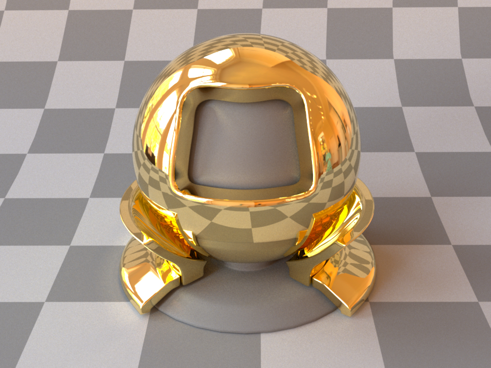
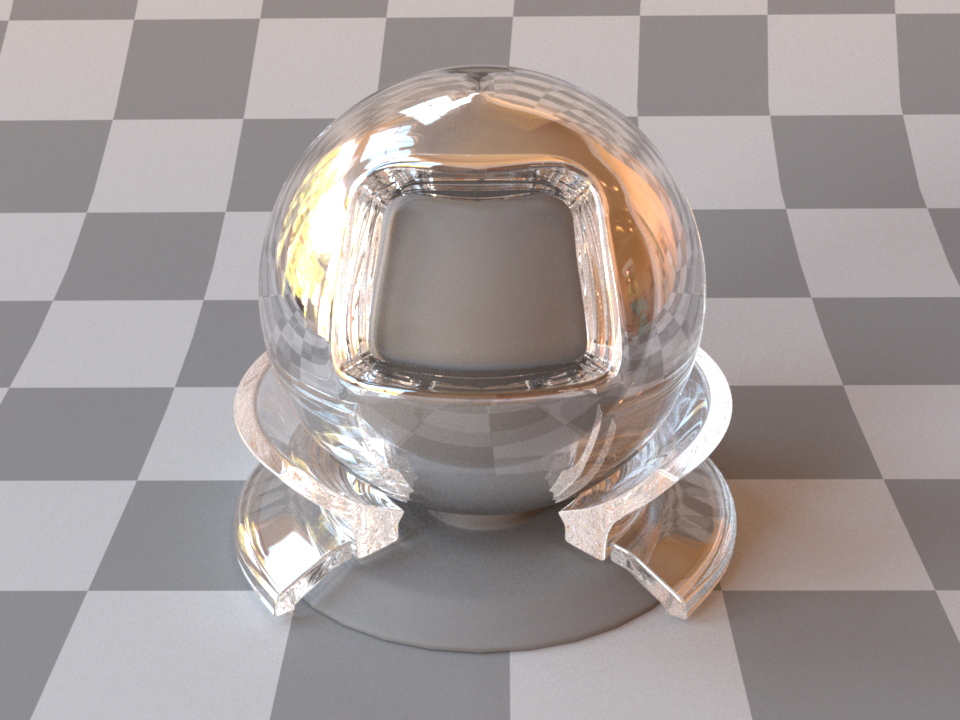
This plugin implements a perfectly smooth interface to a conducting material, such as a metal that is described using a Dirac delta distribution. For a similar model that instead describes a rough surface microstructure, take a look at the separately available roughconductor plugin. In contrast to dielectric materials, conductors do not transmit any light. Their index of refraction is complex-valued and tends to undergo considerable changes throughout the visible color spectrum.

When using this plugin, you should ideally enable one of the spectral modes of the renderer to get the most accurate results. While it also works in RGB mode, the computations will be more approximate in nature. Also note that this material is one-sided—that is, observed from the back side, it will be completely black. If this is undesirable, consider using the twosided BRDF adapter plugin.

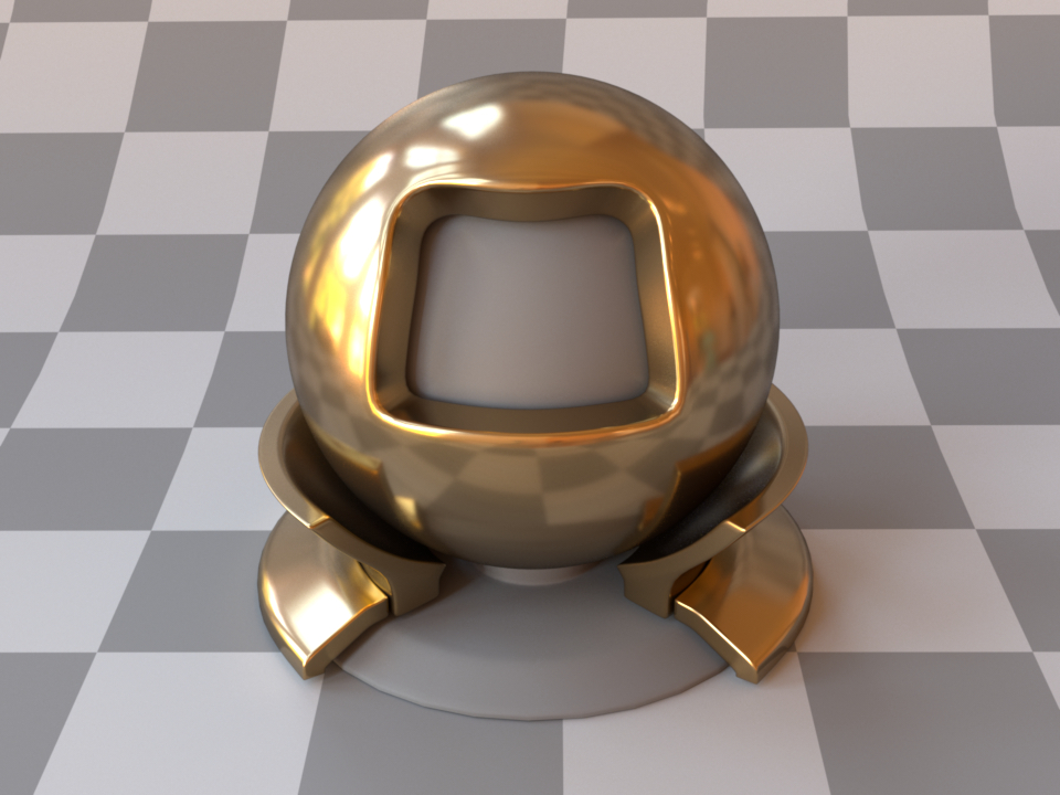
The following XML snippet describes a material definition for gold:

<bsdf type="conductor">
    <string name="material" value="Au"/>
</bsdf>

It is also possible to load spectrally varying index of refraction data from two external files containing the real and imaginary components, respectively (see Scene format for details on the file format):

<bsdf type="conductor">
    <spectrum name="eta" filename="conductorIOR.eta.spd"/>
    <spectrum name="k" filename="conductorIOR.k.spd"/>
</bsdf>

In polarized rendering modes, the material automatically switches to a polarized implementation of the underlying Fresnel equations.

To facilitate the tedious task of specifying spectrally-varying index of refraction information, Mitsuba 2 ships with a set of measured data for several materials, where visible-spectrum information was publicly available:

Preset(s)	Description	Preset(s)	Description
a-C	Amorphous carbon	Na_palik	Sodium
Ag	Silver	Nb, Nb_palik	Niobium
Al	Aluminium	Ni_palik	Nickel
AlAs, AlAs_palik	Cubic aluminium arsenide	Rh, Rh_palik	Rhodium
AlSb, AlSb_palik	Cubic aluminium antimonide	Se, Se_palik	Selenium
Au	Gold	SiC, SiC_palik	Hexagonal silicon carbide
Be, Be_palik	Polycrystalline beryllium	SnTe, SnTe_palik	Tin telluride
Cr	Chromium	Ta, Ta_palik	Tantalum
CsI, CsI_palik	Cubic caesium iodide	Te, Te_palik	Trigonal tellurium
Cu, Cu_palik	Copper	ThF4, ThF4_palik	Polycryst. thorium (IV) fluoride
Cu2O, Cu2O_palik	Copper (I) oxide	TiC, TiC_palik	Polycrystalline titanium carbide
CuO, CuO_palik	Copper (II) oxide	TiN, TiN_palik	Titanium nitride
d-C, d-C_palik	Cubic diamond	TiO2, TiO2_palik	Tetragonal titan. dioxide
Hg, Hg_palik	Mercury	VC, VC_palik	Vanadium carbide
HgTe, HgTe_palik	Mercury telluride	V_palik	Vanadium
Ir, Ir_palik	Iridium	VN, VN_palik	Vanadium nitride
K, K_palik	Polycrystalline potassium	W	Tungsten
Li, Li_palik	Lithium
MgO, MgO_palik	Magnesium oxide
Mo, Mo_palik	Molybdenum	none	No mat. profile (100% reflecting mirror)

This table lists all supported materials that can be passed into the conductor and roughconductor plugins. Note that some of them are not actually conductors—this is not a problem, they can be used regardless (though only the reflection component and no transmission will be simulated). In most cases, there are multiple entries for each material, which represent measurements by different authors.

These index of refraction values are identical to the data distributed with PBRT. They are originally from the Luxpop database and are based on data by Palik et al. [PG98] and measurements of atomic scattering factors made by the Center For X-Ray Optics (CXRO) at Berkeley and the Lawrence Livermore National Laboratory (LLNL).

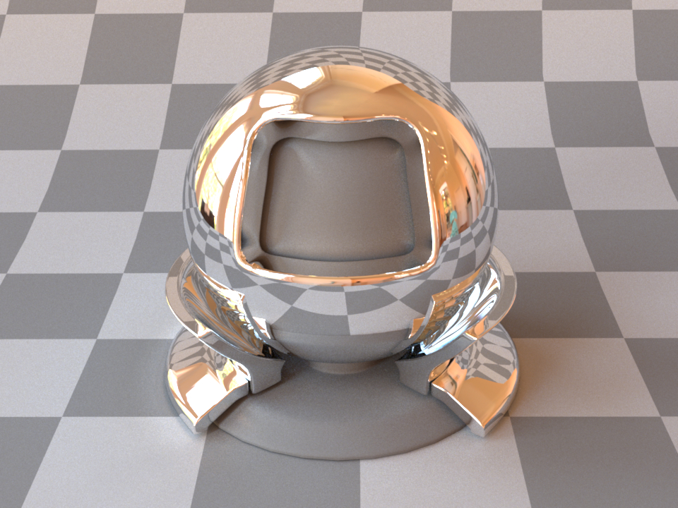
There is also a special material profile named none, which disables the computation of Fresnel reflectances and produces an idealized 100% reflecting mirror.

Rough conductor material (roughconductor)

Parameter	Type	Description
material	string	Name of the material preset, see conductor-ior-list. (Default: none)
eta, k	spectrum or texture	Real and imaginary components of the material’s index of refraction. (Default: based on the value of material)
specular_reflectance	spectrum or texture	Optional factor that can be used to modulate the specular reflection component. Note that for physical realism, this parameter should never be touched. (Default: 1.0)
distribution	string	Specifies the type of microfacet normal distribution used to model the surface roughness. beckmann: Physically-based distribution derived from Gaussian random surfaces. This is the default. ggx: The GGX [WMLT07] distribution (also known as Trowbridge-Reitz [TR75] distribution) was designed to better approximate the long tails observed in measurements of ground surfaces, which are not modeled by the Beckmann distribution.
alpha, alpha_u, alpha_v	texture or float	Specifies the roughness of the unresolved surface micro-geometry along the tangent and bitangent directions. When the Beckmann distribution is used, this parameter is equal to the root mean square (RMS) slope of the microfacets. alpha is a convenience parameter to initialize both alpha_u and alpha_v to the same value. (Default: 0.1)
sample_visible	boolean	Enables a sampling technique proposed by Heitz and D’Eon [HDEon14], which focuses computation on the visible parts of the microfacet normal distribution, considerably reducing variance in some cases. (Default: true, i.e. use visible normal sampling)

This plugin implements a realistic microfacet scattering model for rendering rough conducting materials, such as metals.

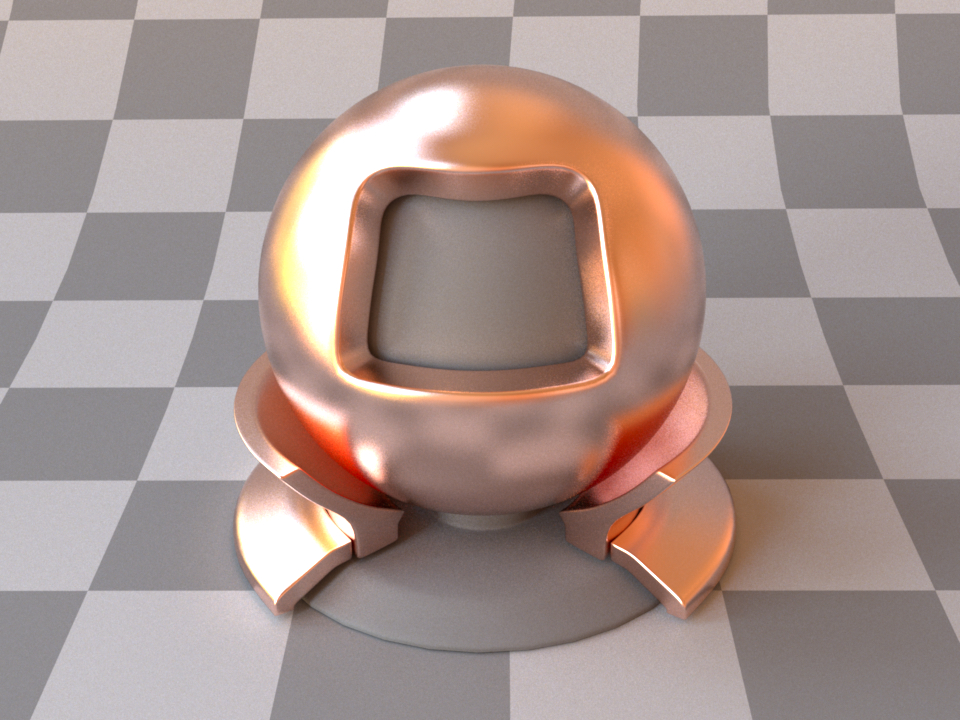
Rough copper (Beckmann, \(\alpha=0.1\))

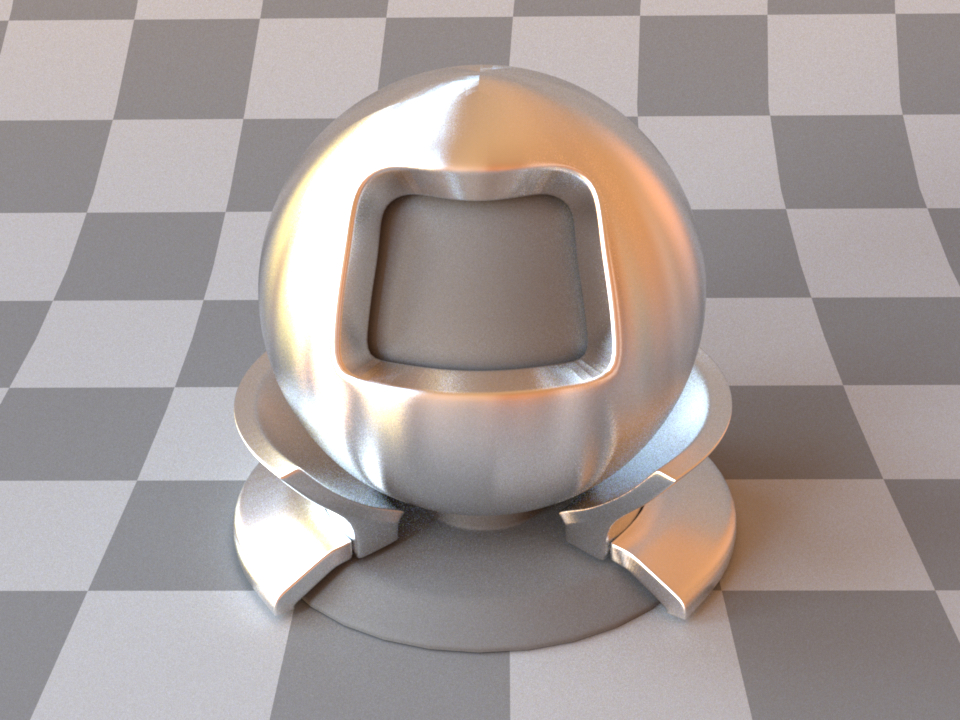
Vertically brushed aluminium (Anisotropic Beckmann, \(\alpha_u=0.05,\ \alpha_v=0.3\))

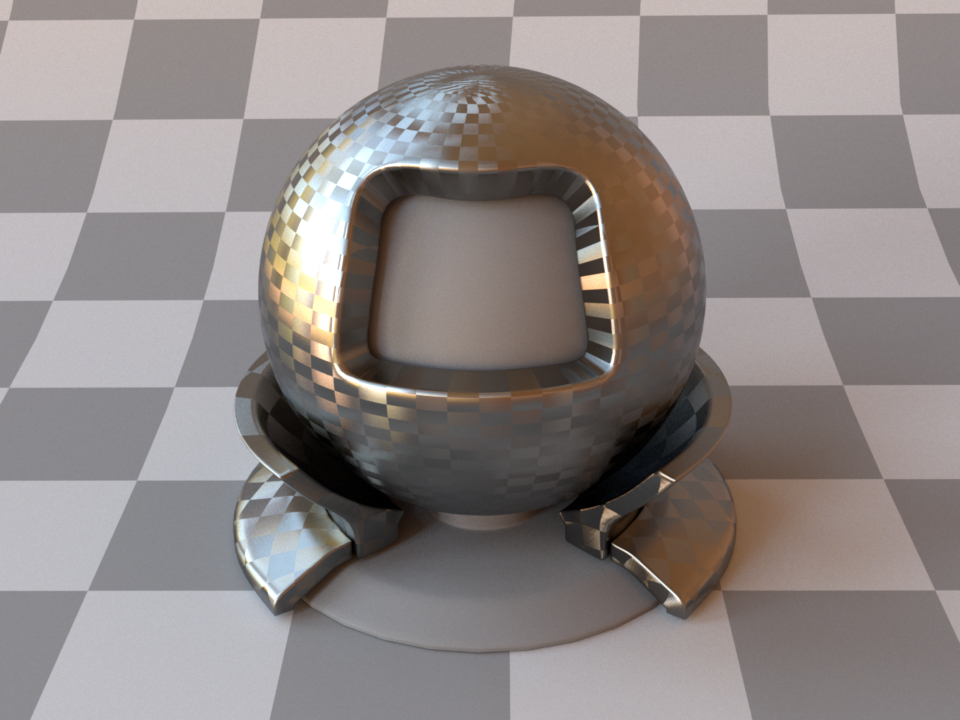
Carbon fiber using two inverted checkerboard textures for alpha_u and alpha_v

Microfacet theory describes rough surfaces as an arrangement of unresolved and ideally specular facets, whose normal directions are given by a specially chosen microfacet distribution. By accounting for shadowing and masking effects between these facets, it is possible to reproduce the important off-specular reflections peaks observed in real-world measurements of such materials.

This plugin is essentially the roughened equivalent of the (smooth) plugin conductor. For very low values of \(\alpha\), the two will be identical, though scenes using this plugin will take longer to render due to the additional computational burden of tracking surface roughness.

The implementation is based on the paper Microfacet Models for Refraction through Rough Surfaces by Walter et al. [WMLT07] and it supports two different types of microfacet distributions.

To facilitate the tedious task of specifying spectrally-varying index of refraction information, this plugin can access a set of measured materials for which visible-spectrum information was publicly available (see the corresponding table in the conductor reference).

When no parameters are given, the plugin activates the default settings, which describe a 100% reflective mirror with a medium amount of roughness modeled using a Beckmann distribution.

To get an intuition about the effect of the surface roughness parameter \(\alpha\), consider the following approximate classification: a value of \(\alpha=0.001-0.01\) corresponds to a material with slight imperfections on an otherwise smooth surface finish, \(\alpha=0.1\) is relatively rough, and \(\alpha=0.3-0.7\) is extremely rough (e.g. an etched or ground finish). Values significantly above that are probably not too realistic.

The following XML snippet describes a material definition for brushed aluminium:

<bsdf type="roughconductor">
    <string name="material" value="Al"/>
    <string name="distribution" value="ggx"/>
    <float name="alphaU" value="0.05"/>
    <float name="alphaV" value="0.3"/>
</bsdf>

Technical details

All microfacet distributions allow the specification of two distinct roughness values along the tangent and bitangent directions. This can be used to provide a material with a brushed appearance. The alignment of the anisotropy will follow the UV parameterization of the underlying mesh. This means that such an anisotropic material cannot be applied to triangle meshes that are missing texture coordinates.

Since Mitsuba 0.5.1, this plugin uses a new importance sampling technique contributed by Eric Heitz and Eugene D’Eon, which restricts the sampling domain to the set of visible (unmasked) microfacet normals. The previous approach of sampling all normals is still available and can be enabled by setting sample_visible to false. However this will lead to significantly slower convergence.

When using this plugin, you should ideally compile Mitsuba with support for spectral rendering to get the most accurate results. While it also works in RGB mode, the computations will be more approximate in nature. Also note that this material is one-sided—that is, observed from the back side, it will be completely black. If this is undesirable, consider using the twosided BRDF adapter.

In polarized rendering modes, the material automatically switches to a polarized implementation of the underlying Fresnel equations.

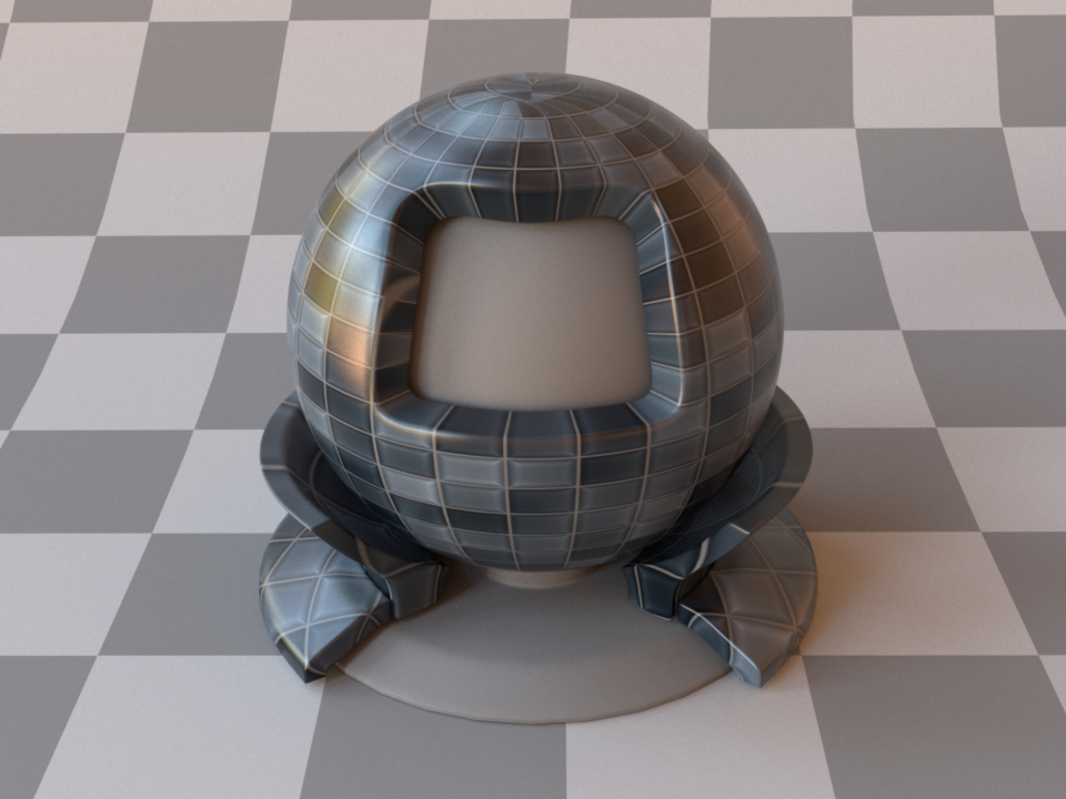
Smooth plastic material (plastic)

Parameter	Type	Description
diffuse_reflectance	spectrum or texture	Optional factor used to modulate the diffuse reflection component. (Default: 0.5)
nonlinear	boolean	Account for nonlinear color shifts due to internal scattering? See the main text for details.. (Default: Don’t account for them and preserve the texture colors, i.e. false)
int_ior	float or string	Interior index of refraction specified numerically or using a known material name. (Default: polypropylene / 1.49)
ext_ior	float or string	Exterior index of refraction specified numerically or using a known material name. (Default: air / 1.000277)
specular_reflectance	spectrum or texture	Optional factor that can be used to modulate the specular reflection component. Note that for physical realism, this parameter should never be touched. (Default: 1.0)

A rendering with the default parameters

A rendering with custom parameters

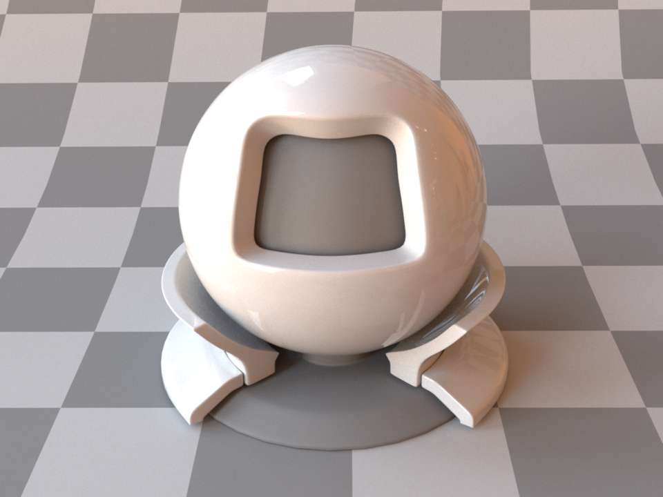
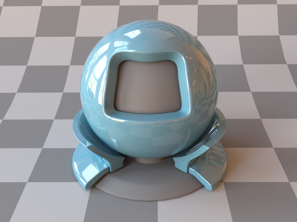
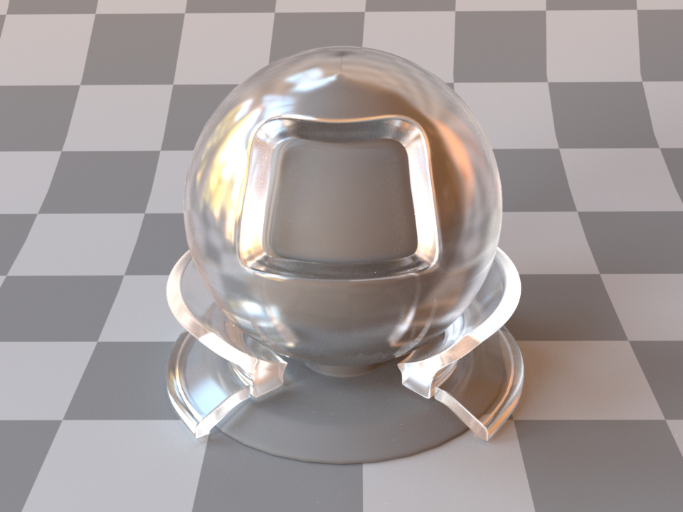
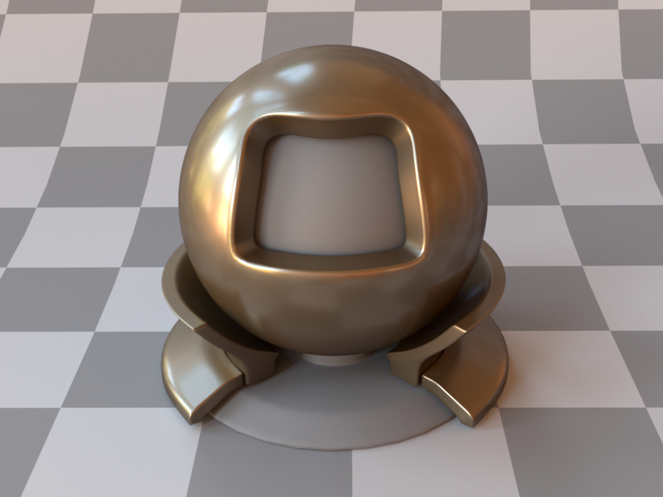
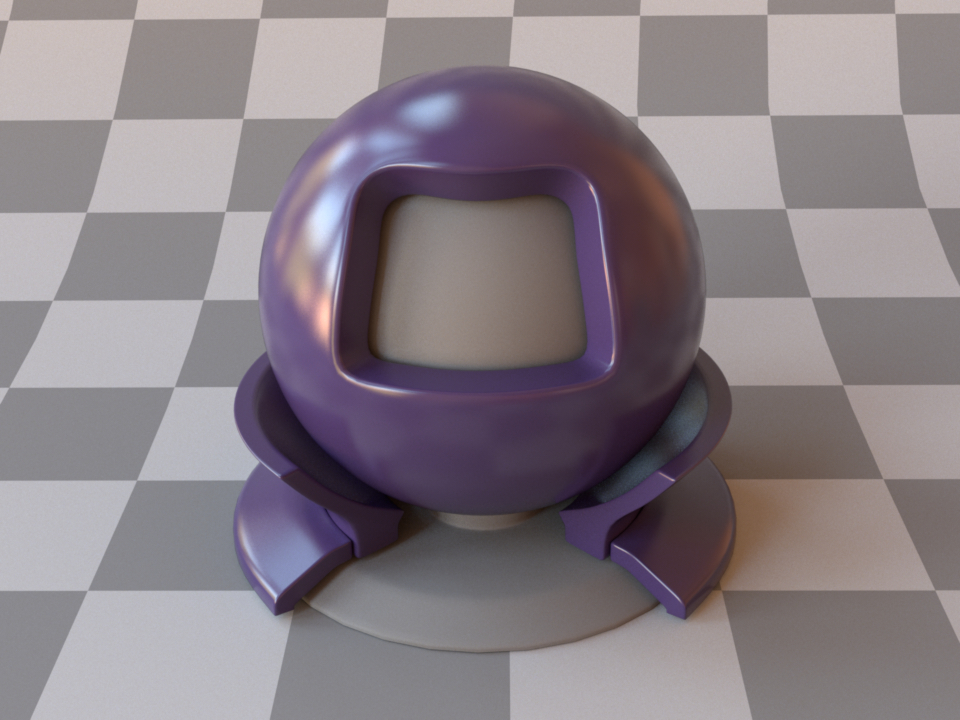
This plugin describes a smooth plastic-like material with internal scattering. It uses the Fresnel reflection and transmission coefficients to provide direction-dependent specular and diffuse components. Since it is simple, realistic, and fast, this model is often a better choice than the roughplastic plugins when rendering smooth plastic-like materials. For convenience, this model allows to specify IOR values either numerically, or based on a list of known materials (see the corresponding table in the dielectric reference). When no parameters are given, the plugin activates the defaults, which describe a white polypropylene plastic material.

The following XML snippet describes a shiny material whose diffuse reflectance is specified using sRGB:

<bsdf type="plastic">
    <rgb name="diffuse_reflectance" value="0.1, 0.27, 0.36"/>
    <float name="int_ior" value="1.9"/>
</bsdf>

Internal scattering

Internally, this model simulates the interaction of light with a diffuse base surface coated by a thin dielectric layer. This is a convenient abstraction rather than a restriction. In other words, there are many materials that can be rendered with this model, even if they might not fit this description perfectly well.

(a) At the boundary, incident illumination is partly reflected and refracted

(b) The refracted portion scatters diffusely at the base layer

(c) An illustration of the scattering events that are internally handled by this plugin

Given illumination that is incident upon such a material, a portion of the illumination is specularly reflected at the material boundary, which results in a sharp reflection in the mirror direction (a). The remaining illumination refracts into the material, where it scatters from the diffuse base layer (b). While some of the diffusely scattered illumination is able to directly refract outwards again, the remainder is reflected from the interior side of the dielectric boundary and will in fact remain trapped inside the material for some number of internal scattering events until it is finally able to escape (c).

Due to the mathematical simplicity of this setup, it is possible to work out the correct form of the model without actually having to simulate the potentially large number of internal scattering events.

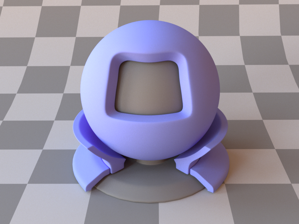
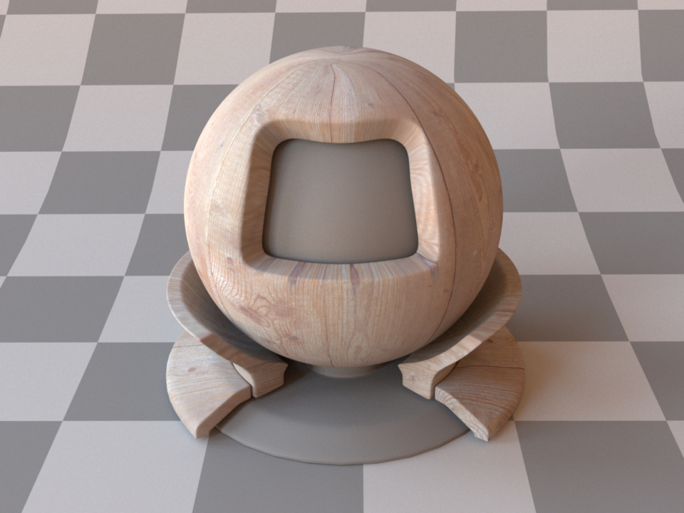
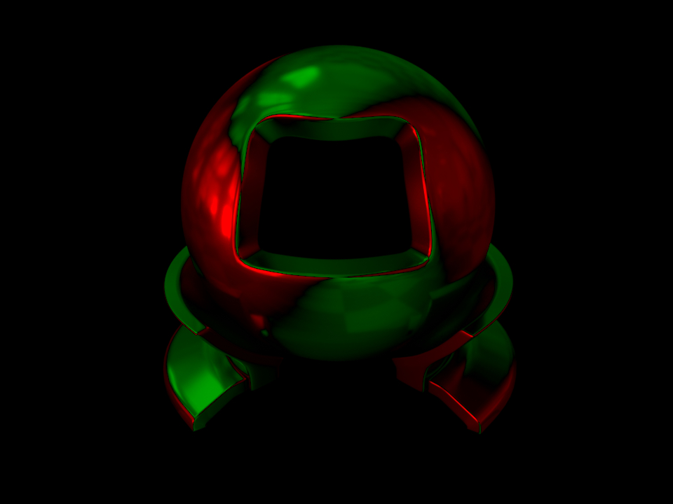
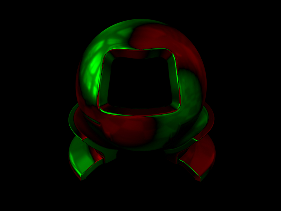
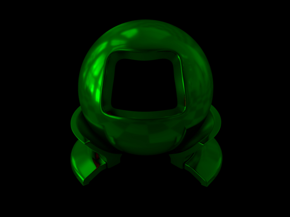
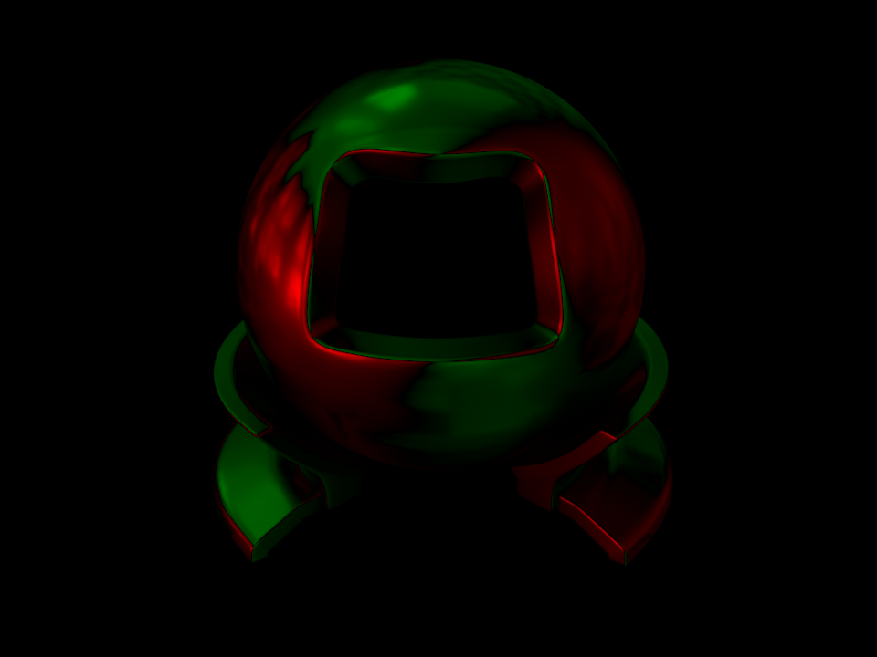
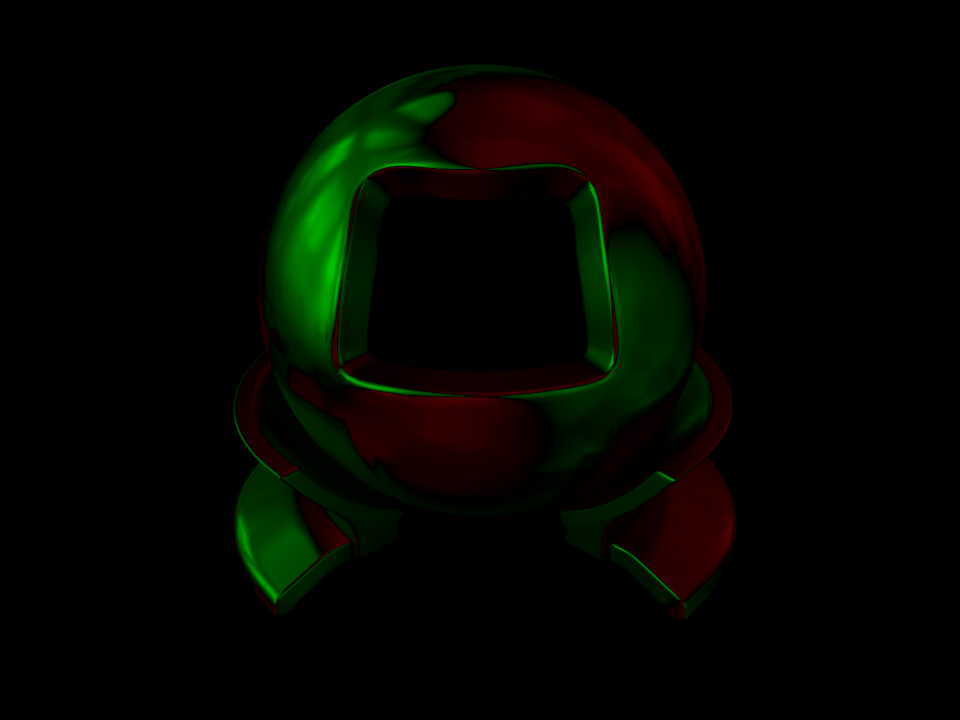
Note that due to the internal scattering, the diffuse color of the material is in practice slightly different from the color of the base layer on its own—in particular, the material color will tend to shift towards darker colors with higher saturation. Since this can be counter-intuitive when using bitmap textures, these color shifts are disabled by default. Specify the parameter nonlinear=true to enable them. The following renderings illustrate the resulting change:

Diffuse textured rendering

Plastic model, nonlinear=false

Plastic model, nonlinear=true

This effect is also seen in real life, for instance a piece of wood will look slightly darker after coating it with a layer of varnish.

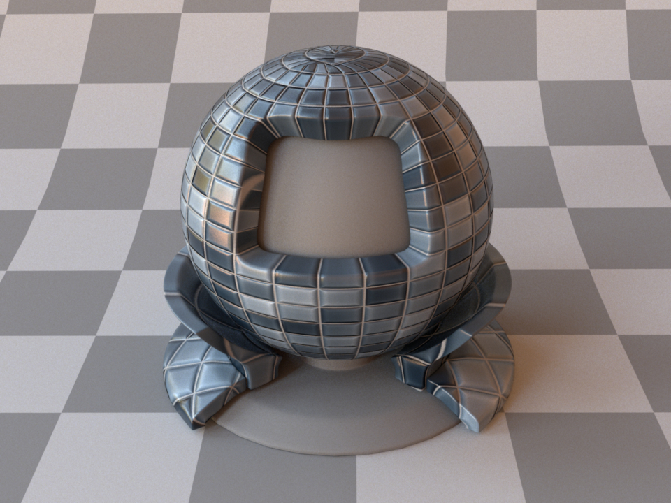
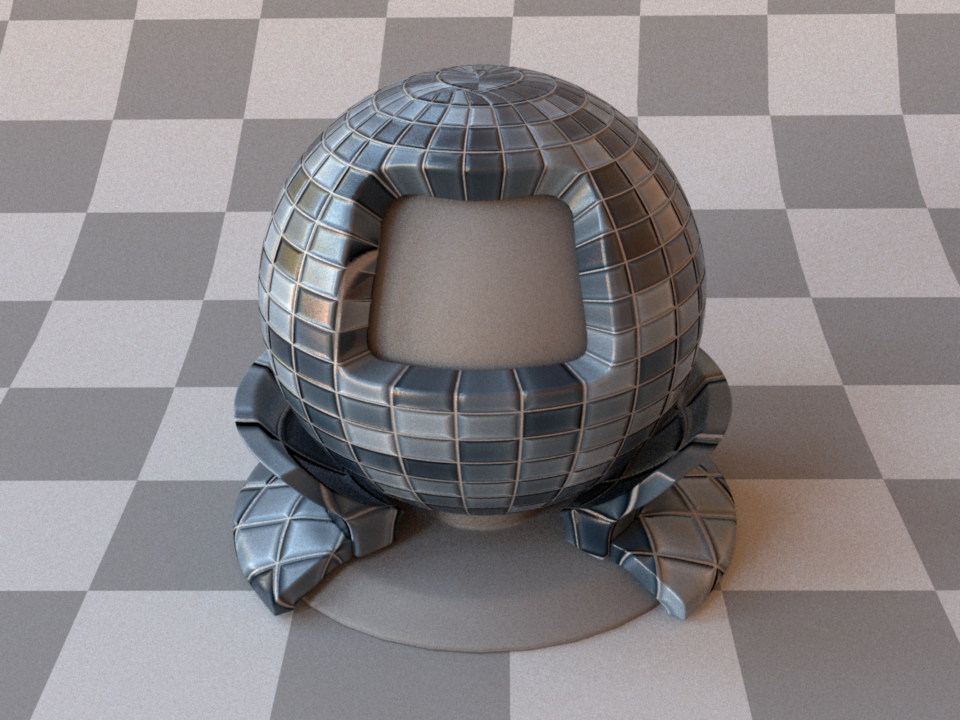
Rough plastic material (roughplastic)

Parameter	Type	Description
diffuse_reflectance	spectrum or texture	Optional factor used to modulate the diffuse reflection component. (Default: 0.5)
nonlinear	boolean	Account for nonlinear color shifts due to internal scattering? See the plastic plugin for details. default{Don’t account for them and preserve the texture colors. (Default: false)
int_ior	float or string	Interior index of refraction specified numerically or using a known material name. (Default: polypropylene / 1.49)
ext_ior	float or string	Exterior index of refraction specified numerically or using a known material name. (Default: air / 1.000277)
specular_reflectance	spectrum or texture	Optional factor that can be used to modulate the specular reflection component. Note that for physical realism, this parameter should never be touched. (Default: 1.0)
distribution	string	Specifies the type of microfacet normal distribution used to model the surface roughness. beckmann: Physically-based distribution derived from Gaussian random surfaces. This is the default. ggx: The GGX [WMLT07] distribution (also known as Trowbridge-Reitz [TR75] distribution) was designed to better approximate the long tails observed in measurements of ground surfaces, which are not modeled by the Beckmann distribution.
alpha	float	Specifies the roughness of the unresolved surface micro-geometry along the tangent and bitangent directions. When the Beckmann distribution is used, this parameter is equal to the root mean square (RMS) slope of the microfacets. (Default: 0.1)
sample_visible	boolean	Enables a sampling technique proposed by Heitz and D’Eon [HDEon14], which focuses computation on the visible parts of the microfacet normal distribution, considerably reducing variance in some cases. (Default: true, i.e. use visible normal sampling)

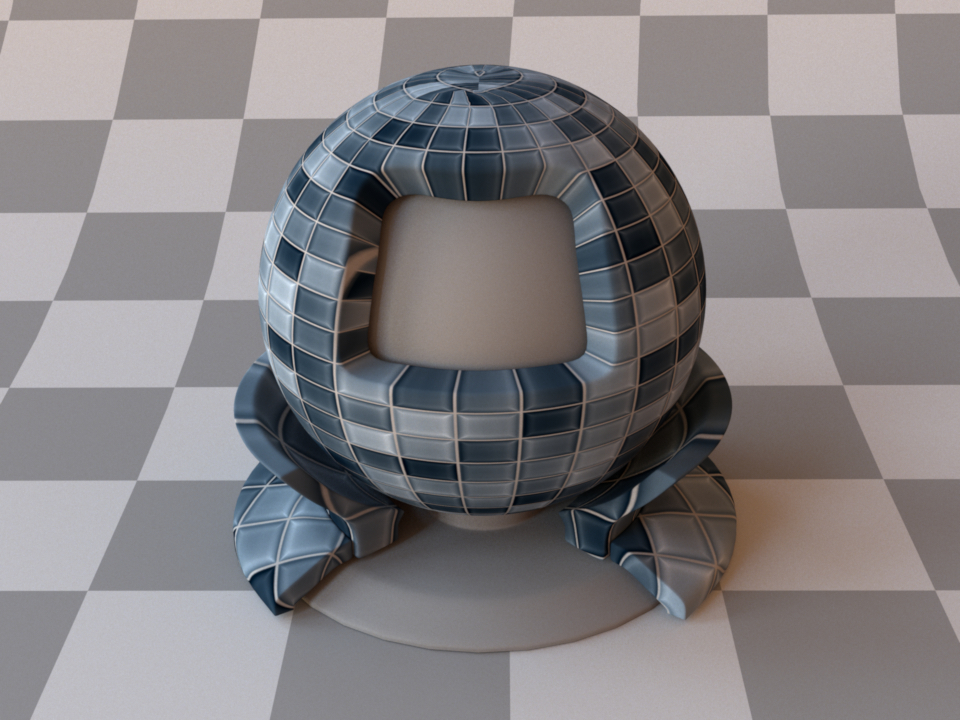
This plugin implements a realistic microfacet scattering model for rendering rough dielectric materials with internal scattering, such as plastic.

Microfacet theory describes rough surfaces as an arrangement of unresolved and ideally specular facets, whose normal directions are given by a specially chosen microfacet distribution. By accounting for shadowing and masking effects between these facets, it is possible to reproduce the important off-specular reflections peaks observed in real-world measurements of such materials.

Beckmann, \(\alpha=0.1\)

GGX, \(\alpha=0.3\)

This plugin is essentially the roughened equivalent of the (smooth) plugin plastic. For very low values of \(\alpha\), the two will be identical, though scenes using this plugin will take longer to render due to the additional computational burden of tracking surface roughness.

For convenience, this model allows to specify IOR values either numerically, or based on a list of known materials (see the corresponding table in the dielectric reference). When no parameters are given, the plugin activates the defaults, which describe a white polypropylene plastic material with a light amount of roughness modeled using the Beckmann distribution.

To get an intuition about the effect of the surface roughness parameter \(\alpha\), consider the following approximate classification: a value of \(\alpha=0.001-0.01\) corresponds to a material with slight imperfections on an otherwise smooth surface finish, \(\alpha=0.1\) is relatively rough, and \(\alpha=0.3-0.7\) is extremely rough (e.g. an etched or ground finish). Values significantly above that are probably not too realistic.

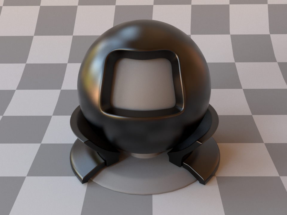
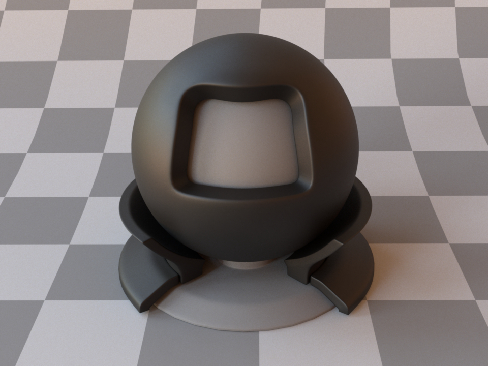
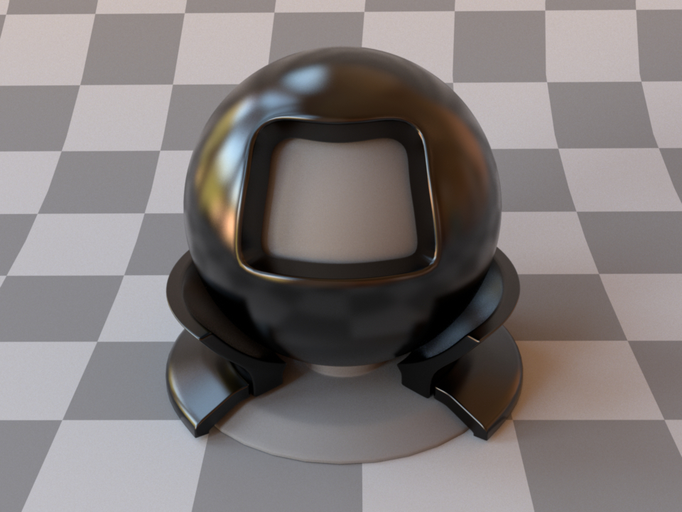
The following XML snippet describes a material definition for black plastic material.

<bsdf type="roughplastic">
    <string name="distribution" value="beckmann"/>
    <float name="int_ior" value="1.61"/>
    <spectrum name="diffuse_reflectance" value="0"/>
</bsdf>

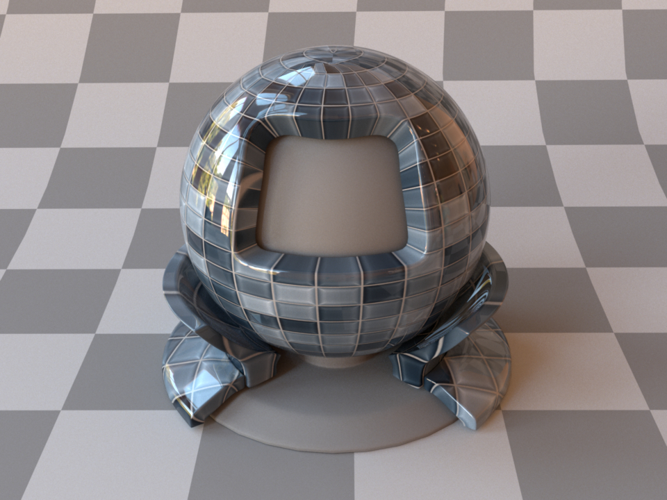
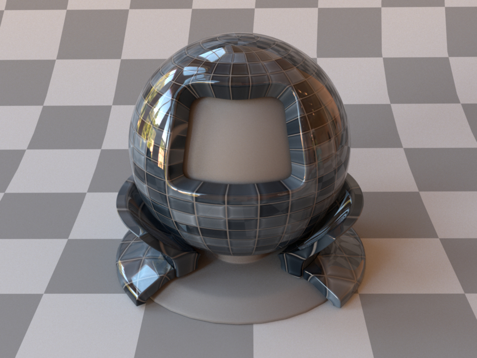
Like the plastic material, this model internally simulates the interaction of light with a diffuse base surface coated by a thin dielectric layer (where the coating layer is now rough). This is a convenient abstraction rather than a restriction. In other words, there are many materials that can be rendered with this model, even if they might not fit this description perfectly well.

The simplicity of this setup makes it possible to account for interesting nonlinear effects due to internal scattering, which is controlled by the nonlinear parameter:

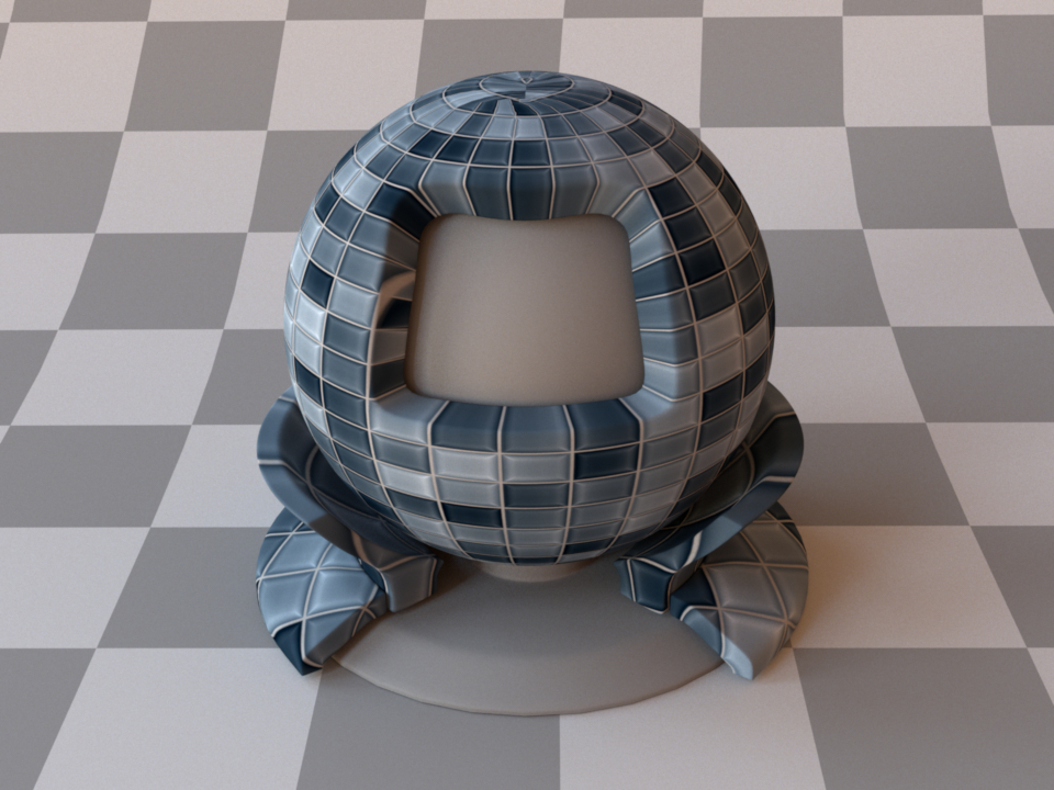
Diffuse textured rendering

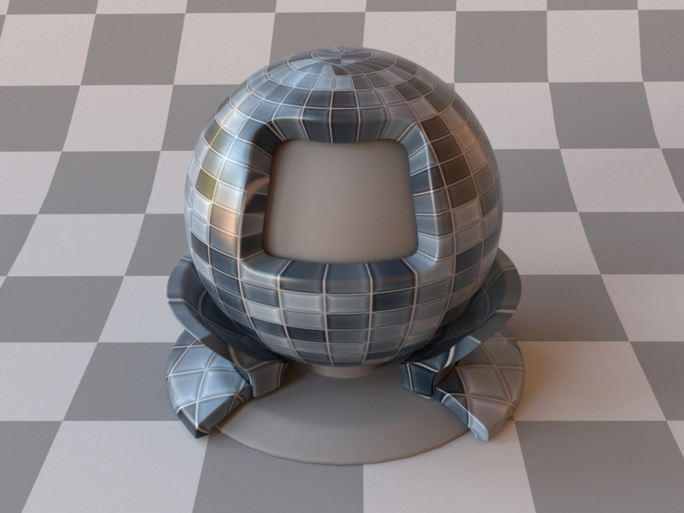
Rough plastic model with nonlinear=false

Textured rough plastic model with nonlinear=true

For more details, please refer to the description of this parameter given in the plastic plugin section.

Bump map BSDF adapter (bumpmap)

Parameter	Type	Description
(Nested plugin)	texture	Specifies the bump map texture.
(Nested plugin)	bsdf	A BSDF model that should be affected by the bump map
scale	float	Bump map gradient multiplier. (Default: 1.0)

Bump mapping is a simple technique for cheaply adding surface detail to a rendering. This is done by perturbing the shading coordinate frame based on a displacement height field provided as a texture. This method can lend objects a highly realistic and detailed appearance (e.g. wrinkled or covered by scratches and other imperfections) without requiring any changes to the input geometry. The implementation in Mitsuba uses the common approach of ignoring the usually negligible texture-space derivative of the base mesh surface normal. As side effect of this decision, it is invariant to constant offsets in the height field texture: only variations in its luminance cause changes to the shading frame.

Note that the magnitude of the height field variations influences the scale of the displacement.

Roughplastic BSDF

Roughplastic BSDF with bump mapping

The following XML snippet describes a rough plastic material affected by a bump map. Note the we set the raw properties of the bump map bitmap object to true in order to disable the transformation from sRGB to linear encoding:

<bsdf type="bumpmap">
    <texture name="arbitrary" type="bitmap">
        <boolean name="raw" value="true"/>
        <string name="filename" value="textures/bumpmap.jpg"/>
    </texture>
    <bsdf type="roughplastic"/>
</bsdf>

Normal map BSDF (normalmap)

Parameter	Type	Description
normalmap	texture	The color values of this texture specify the perturbed normals relative in the local surface coordinate system
(Nested plugin)	bsdf	A BSDF model that should be affected by the normal map

Normal mapping is a simple technique for cheaply adding surface detail to a rendering. This is done by perturbing the shading coordinate frame based on a normal map provided as a texture. This method can lend objects a highly realistic and detailed appearance (e.g. wrinkled or covered by scratches and other imperfections) without requiring any changes to the input geometry.

Roughplastic BSDF

Roughplastic BSDF with normal mapping

A normal map is a RGB texture, whose color channels encode the XYZ coordinates of the desired surface normals. These are specified relative to the local shading frame, which means that a normal map with a value of \((0,0,1)\) everywhere causes no changes to the surface. To turn the 3D normal directions into (nonnegative) color values suitable for this plugin, the mapping \(x \mapsto (x+1)/2\) must be applied to each component.

The following XML snippet describes a smooth mirror material affected by a normal map. Note the we set the raw properties of the normal map bitmap object to true in order to disable the transformation from sRGB to linear encoding:

<bsdf type="normalmap">
    <texture name="normalmap" type="bitmap">
        <boolean name="raw" value="true"/>
        <string name="filename" value="textures/normalmap.jpg"/>
    </texture>
    <bsdf type="roughplastic"/>
</bsdf>

Blended material (blendbsdf)

Parameter	Type	Description
weight	float or texture	A floating point value or texture with values between zero and one. The extreme values zero and one activate the first and second nested BSDF respectively, and inbetween values interpolate accordingly. (Default: 0.5)
(Nested plugin)	bsdf	Two nested BSDF instances that should be mixed according to the specified blending weight

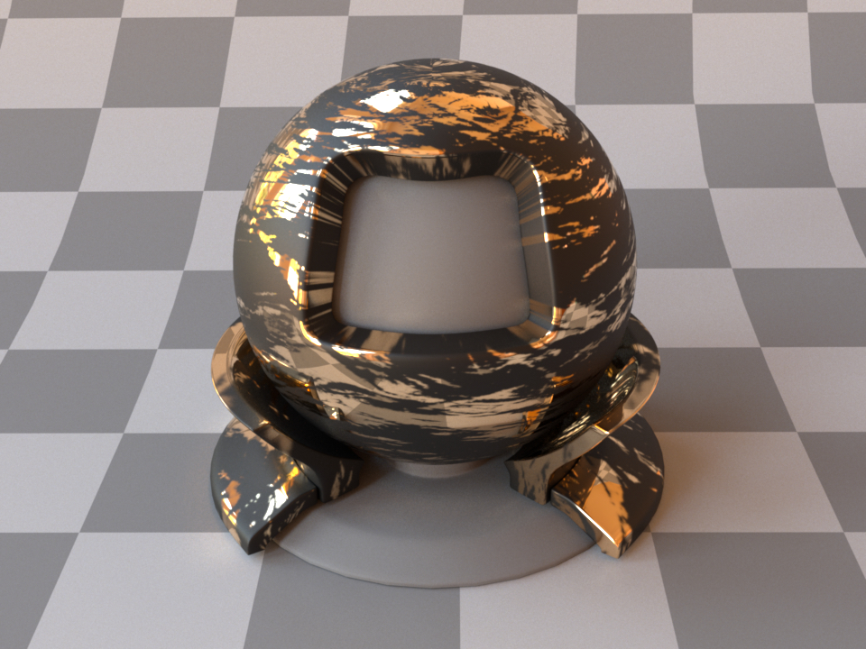
A material created by blending between rough plastic and smooth metal based on a binary bitmap texture

This plugin implements a blend material, which represents linear combinations of two BSDF instances. Any surface scattering model in Mitsuba 2 (be it smooth, rough, reflecting, or transmitting) can be mixed with others in this manner to synthesize new models.

The following XML snippet describes the material shown above:

<bsdf type="blendbsdf">
    <texture name="weight" type="bitmap">
        <string name="filename" value="pattern.png"/>
    </texture>
    <bsdf type="conductor">
    </bsdf>
    <bsdf type="roughplastic">
        <spectrum name="diffuse_reflectance" value="0.1"/>
    </bsdf>
</bsdf>

Opacity mask (mask)

Parameter	Type	Description
opacity	spectrum or texture	Specifies the opacity (where 1=completely opaque) (Default: 0.5)
(Nested plugin)	bsdf	A base BSDF model that represents the non-transparent portion of the scattering

Rendering without an opacity mask

Rendering with an opacity mask

This plugin applies an opacity mask to add nested BSDF instance. It interpolates between perfectly transparent and completely opaque based on the opacity parameter.

The transparency is internally implemented as a forward-facing Dirac delta distribution. Note that the standard path tracer does not have a good sampling strategy to deal with this, but the (volumetric path tracer) does. It may thus be preferable when rendering scenes that contain the mask plugin, even if there is nothing volumetric in the scene.

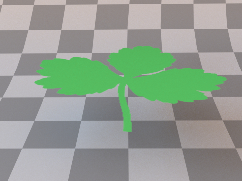
The following XML snippet describes a material configuration for a transparent leaf:

<bsdf type="mask">
    <!-- Base material: a two-sided textured diffuse BSDF -->
    <bsdf type="twosided">
        <bsdf type="diffuse">
            <texture name="reflectance" type="bitmap">
                <string name="filename" value="leaf.png"/>
            </texture>
        </bsdf>
    </bsdf>

    <!-- Fetch the opacity mask from a monochromatic texture -->
    <texture type="bitmap" name="opacity">
        <string name="filename" value="leaf_mask.png"/>
    </texture>
</bsdf>

Two-sided BRDF adapter (twosided)

Parameter	Type	Description
(Nested plugin)	bsdf	A nested BRDF that should be turned into a two-sided scattering model. If two BRDFs are specified, they will be placed on the front and back side, respectively

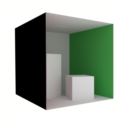
From this angle, the Cornell box scene shows visible back-facing geometry

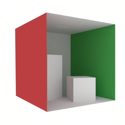
Applying the twosided plugin fixes the rendering

By default, all non-transmissive scattering models in Mitsuba 2 are one-sided — in other words, they absorb all light that is received on the interior-facing side of any associated surfaces. Holes and visible back-facing parts are thus exposed as black regions.

Usually, this is a good idea, since it will reveal modeling issues early on. But sometimes one is forced to deal with improperly closed geometry, where the one-sided behavior is bothersome. In that case, this plugin can be used to turn one-sided scattering models into proper two-sided versions of themselves. The plugin has no parameters other than a required nested BSDF specification. It is also possible to supply two different BRDFs that should be placed on the front and back side, respectively.

The following snippet describes a two-sided diffuse material:

<bsdf type="twosided">
    <bsdf type="diffuse">
         <spectrum name="reflectance" value="0.4"/>
    </bsdf>
</bsdf>

Null material (null)

This plugin models a completely invisible surface material. Light will not interact with this BSDF in any way.

Internally, this is implemented as a forward-facing Dirac delta distribution. Note that the standard path tracer does not have a good sampling strategy to deal with this, but the (volumetric path tracer) does.

The main purpose of this material is to be used as the BSDF of a shape enclosing a participating medium.

Linear polarizer material (polarizer)

Parameter	Type	Description
theta	spectrum or texture	Specifies the rotation angle (in degrees) of the polarizer around the optical axis (Default: 0.0)
transmittance	spectrum or texture	Optional factor that can be used to modulate the specular transmission. (Default: 1.0)
polarizing	boolean	Optional flag to disable polarization changes in order to use this as a neutral density filter, even in polarized render modes. (Default: true, i.e. act as polarizer)

This material simulates an ideal linear polarizer useful to test polarization aware light transport or to conduct virtual optical experiments. The aborbing axis of the polarizer is aligned with the V-direction of the underlying surface parameterization. To rotate the polarizer, either the parameter theta can be used, or alternative a rotation can be applied directly to the associated shape.

Two aligned polarizers. The average intensity is reduced by a factor of 2.

Two polarizers offset by 90 degrees. All trasmitted light is aborbed.

Two polarizers offset by 90 degrees, with a third polarizer in between at 45 degrees. Some light is transmitted again.

The following XML snippet describes a linear polarizer material with a rotation of 90 degrees.

<bsdf type="polarizer">
    <spectrum name="theta" value="90"/>
</bsdf>

Apart from a change of polarization, light does not interact with this material in any way and does not change its direction. Internally, this is implemented as a forward-facing Dirac delta distribution. Note that the standard path tracer does not have a good sampling strategy to deal with this, but the (volumetric path tracer) does.

In unpolarized rendering modes, the behaviour defaults to a non-polarizing transmitting material that absorbs 50% of the incident illumination.

Linear retarder material (retarder)

Parameter	Type	Description
theta	spectrum or texture	Specifies the rotation angle (in degrees) of the retarder around the optical axis (Default: 0.0)
delta	spectrum or texture	Specifies the retardance (in degrees) where 360 degrees is equivalent to a full wavelength. (Default: 90.0)
transmittance	spectrum or texture	Optional factor that can be used to modulate the specular transmission. (Default: 1.0)

This material simulates an ideal linear retarder useful to test polarization aware light transport or to conduct virtual optical experiments. The fast axis of the retarder is aligned with the U-direction of the underlying surface parameterization. For non-perpendicular incidence, a cosine falloff term is applied to the retardance.

This plugin can be used to instantiate the common special cases of half-wave plates (with delta=180) and quarter-wave plates (with delta=90).

The following XML snippet describes a quarter-wave plate material:

<bsdf type="retarder">
    <spectrum name="delta" value="90"/>
</bsdf>

Apart from a change of polarization, light does not interact with this material in any way and does not change its direction. Internally, this is implemented as a forward-facing Dirac delta distribution. Note that the standard path tracer does not have a good sampling strategy to deal with this, but the (volumetric path tracer) does.

In unpolarized rendering modes, the behaviour defaults to non-polarizing transparent material similar to the null BSDF plugin.

Circular polarizer material (circular)

Parameter	Type	Description
theta	spectrum or texture	Specifies the rotation angle (in degrees) of the polarizer around the optical axis (Default: 0.0)
transmittance	spectrum or texture	Optional factor that can be used to modulate the specular transmission. (Default: 1.0)
left_handed	boolean	Flag to switch between left and right circular polarization. (Default: false, i.e. right circular polarizer)

This material simulates an ideal circular polarizer useful to test polarization aware light transport or to conduct virtual optical experiments. To rotate the polarizer, either the parameter theta can be used, or alternative a rotation can be applied directly to the associated shape.

The following XML snippet describes a left circular polarizer material:

<bsdf type="circular">
    <boolean name="left_handed" value="true"/>
</bsdf>

Apart from a change of polarization, light does not interact with this material in any way and does not change its direction. Internally, this is implemented as a forward-facing Dirac delta distribution. Note that the standard path tracer does not have a good sampling strategy to deal with this, but the (volumetric path tracer) does.

In unpolarized rendering modes, the behaviour defaults to non-polarizing transparent material similar to the null BSDF plugin.

Measured polarized material (measured_polarized)

Parameter	Type	Description
filename	string	Filename of the material data file to be loaded
alpha_sample	float	Specifies which roughness value should be used for the internal Microfacet importance sampling routine. (Default: 0.1)
wavelength	float	Specifies if the material should only be rendered for just one specific wavelength. The valid range is between 450 and 650 nm. A value of -1 means the full spectrally-varying pBRDF will be used. (Default: -1, i.e. all wavelengths.)

This plugin allows rendering of polarized materials (pBRDFs) acquired as part of “Image-Based Acquisition and Modeling of Polarimetric Reflectance” by Baek et al. 2020 ([BZK+20]). The required files for each material can be found in the corresponding database.

The dataset is made out of isotropic pBRDFs spanning a wide range of appearances: diffuse/specular, metallic/dielectric, rough/smooth, and different color albedos, captured in five wavelength ranges covering the visible spectrum from 450 to 650 nm.

Here are two example materials of gold, and a dielectric “fake” gold, together with visualizations of the resulting Stokes vectors rendered with the Stokes integrator:

Measured gold material

“\(\mathbf{s}_1\)”: horizontal vs. vertical polarization

“\(\mathbf{s}_2\)”: positive vs. negative diagonal polarization

“\(\mathbf{s}_3\)”: right vs. left circular polarization

Measured “fake” gold material

“\(\mathbf{s}_1\)”: horizontal vs. vertical polarization

“\(\mathbf{s}_2\)”: positive vs. negative diagonal polarization

“\(\mathbf{s}_3\)”: right vs. left circular polarization

In the following example, the measured gold BSDF from the dataset is setup:

<bsdf type="measured_polarized">
    <string name="filename" value="6_gold_inpainted.pbsdf"/>
    <float name="alpha_sample" value="0.02"/>
</bsdf>

Internally, a sampling routine from the GGX Microfacet model is used in order to importance sampling outgoing directions. The used GGX roughness value is exposed here as a user parameter alpha_sample and should be set according to the approximate roughness of the material to be rendered. Note that any value here will result in a correct rendering but the level of noise can vary significantly.

Polarized plastic material (pplastic)

Parameter	Type	Description
diffuse_reflectance	spectrum or texture	Optional factor used to modulate the diffuse reflection component. (Default: 0.5)
specular_reflectance	spectrum or texture	Optional factor that can be used to modulate the specular reflection component. Note that for physical realism, this parameter should never be touched. (Default: 1.0)
int_ior	float or string	Interior index of refraction specified numerically or using a known material name. (Default: polypropylene / 1.49)
ext_ior	float or string	Exterior index of refraction specified numerically or using a known material name. (Default: air / 1.000277)
distribution	string	Specifies the type of microfacet normal distribution used to model the surface roughness. beckmann: Physically-based distribution derived from Gaussian random surfaces. This is the default. ggx: The GGX [WMLT07] distribution (also known as Trowbridge-Reitz [TR75] distribution) was designed to better approximate the long tails observed in measurements of ground surfaces, which are not modeled by the Beckmann distribution.
alpha	float	Specifies the roughness of the unresolved surface micro-geometry along the tangent and bitangent directions. When the Beckmann distribution is used, this parameter is equal to the root mean square (RMS) slope of the microfacets. (Default: 0.1)
sample_visible	boolean	Enables a sampling technique proposed by Heitz and D’Eon [HDEon14], which focuses computation on the visible parts of the microfacet normal distribution, considerably reducing variance in some cases. (Default: true, i.e. use visible normal sampling)

This plugin implements a scattering model that combines diffuse and specular reflection where both components can interact with polarized light. This is based on the pBRDF proposed in “Simultaneous Acquisition of Polarimetric SVBRDF and Normals” by Baek et al. 2018 ([BJTK18]).

Apart from the polarization support, this is similar to the plastic and roughplastic plugins. There, the interaction of light with a diffuse base surface coated by a (potentially rough) thin dielectric layer is used as a way of combining the two components, whereas here the two are added in a more ad-hoc way:

1. The specular component is a standard rough reflection from a microfacet model.

2. The diffuse Lambert component is attenuated by a smooth refraction into and out of the material where conceptually some subsurface scattering occurs in between that causes the light to escape in a diffused way.

This is illusrated in the following diagram:

The intensity of the rough reflection is always less than the light lost by the two refractions which means the addition of these components does not result in any extra energy. However, it is also not energy conserving.

What makes this plugin particularly interesting is that both components account for the polarization state of light when it interacts with the material. For applications without the need of polarization support, it is recommended to stick to the standard plastic and roughplastic plugins.

See the following images of the two components rendered individually together with false-color visualizations of the resulting “\(\mathbf{s}_1\)” Stokes vector output that encodes horizontal vs. vertical linear polarization.

Specular component

Diffuse component

“\(\mathbf{s}_1\)” for the specular component

“\(\mathbf{s}_1\)” for the diffuse component

Note how the diffuse polarization is comparatively weak and has its orientation flipped by 90 degrees. This is a property that is commonly exploited in shape from polarization applications ([KTSR17]).

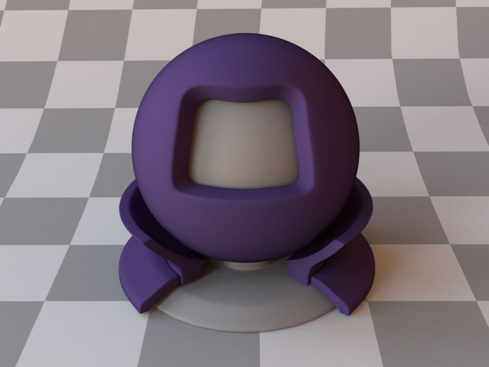
The following XML snippet describes the purple material from the test scene above:

<bsdf type="pplastic">
    <rgb name="diffuse_reflectance" value="0.05, 0.03, 0.1"/>
    <float name="alpha" value="0.06"/>
</bsdf>

Bi-Lambertian material (bilambertian)

Parameter	Type	Description
reflectance	spectrum or texture	Specifies the diffuse reflectance of the material (Default: 0.5)
transmittance	spectrum or texture	Specifies the diffuse transmittance of the material (Default: 0.5)

The bi-Lambertian material represents a material that scatters light diffusely into the entire sphere. The reflectance specifies the amount of light scattered into the incoming hemisphere, while the transmittance specifies the amount of light scattered into the outgoing hemisphere. This material is two-sided.

With dominant reflectivity

With dominant transmissivity

Rahman Pinty Verstraete reflection model (rpv)

Parameter	Type	Description
rho_0	spectrum or texture	\(\rho_0 \ge 0\). Default: 0.1
k	spectrum or texture	\(k \in \mathbb{R}\). Default: 0.1
g	spectrum or texture	\(-1 \le g \le 1\). Default: 0.0
rho_c	spectrum or texture	Default: Equal to rho_0

This plugin implements the reflection model proposed by [RPV93].

Apart from homogeneous values, the plugin can also accept nested or referenced texture maps to be used as the source of parameter information, which is then mapped onto the shape based on its UV parameterization. When no parameters are specified, the model uses the default values of \(\rho_0 = 0.1\), \(k = 0.1\) and \(g = 0.0\)

This plugin also supports the most common extension to four parameters, namely the \(\rho_c\) extension, as used in [WLP+06].

For the fundamental formulae defining the RPV model please refer to the Eradiate Scientific Handbook.

Note that this material is one-sided, that is, observed from the back side, it will be completely black. If this is undesirable, consider using the twosided BRDF adapter plugin. The following XML snippet describes an RPV material with monochromatic parameters:

<bsdf type="rpv">
    <float name="rho_0" value="0.02"/>
    <float name="k" value="0.3"/>
    <float name="g" value="-0.12"/>
</bsdf>

Phase functions

This section contains a description of all implemented medium scattering models, which are also known as phase functions. These are very similar in principle to surface scattering models (or BSDFs), and essentially describe where light travels after hitting a particle within the medium. Currently, only the most commonly used models for smoke, fog, and other homogeneous media are implemented.

Isotropic phase function (isotropic)

This phase function simulates completely uniform scattering, where all directionality is lost after a single scattering interaction. It does not have any parameters.

Henyey-Greenstein phase function (hg)

Parameter	Type	Description
g	float	This parameter must be somewhere in the range -1 to 1 (but not equal to -1 or 1). It denotes the mean cosine of scattering interactions. A value greater than zero indicates that medium interactions predominantly scatter incident light into a similar direction (i.e. the medium is forward-scattering), whereas values smaller than zero cause the medium to be scatter more light in the opposite direction.

This plugin implements the phase function model proposed by Henyey and Greenstein [HG41]. It is parameterizable from backward- (g<0) through isotropic- (g=0) to forward (g>0) scattering.

Tabulated phase function (tabphase)

Parameter	Type	Description
values	string	A comma-separated list of phase function values parametrised by the cosine of the scattering angle.

This plugin implements a generic phase function model for isotropic media parametrised by a lookup table giving values of the phase function as a function of the cosine of the scattering angle.

Notes

• The scattering angle is here defined as the dot product of the incoming and outgoing directions, where the incoming, resp. outgoing direction points toward, resp. outward the interaction point.

• From this follows that \(\cos \theta = 1\) corresponds to forward scattering.

• Lookup table points are regularly spaced between -1 and 1.

• Phase function values are automatically normalized.

Blended phase function (blendphase)

Parameter	Type	Description
weight	float or texture	A floating point value or texture with values between zero and one. The extreme values zero and one activate the first and second nested phase function respectively, and inbetween values interpolate accordingly. (Default: 0.5)
(Nested plugin)	|phase|	Two nested phase function instances that should be mixed according to the specified blending weight

This plugin implements a blend phase function, which represents linear combinations of two phase function instances. Any phase function in Mitsuba 2 (be it isotropic, anisotropic, micro-flake …) can be mixed with others in this manner. This is of particular interest when mixing components in a participating medium (e.g. accounting for the presence of aerosols in a Rayleigh-scattering atmosphere).

Rayleigh phase function (rayleigh)

Scattering by particles that are much smaller than the wavelength of light (e.g. individual molecules in the atmosphere) is well-approximated by the Rayleigh phase function. This plugin implements an unpolarized version of this scattering model (i.e. the effects of polarization are ignored). This plugin is useful for simulating scattering in planetary atmospheres.

This model has no parameters.

Emitters

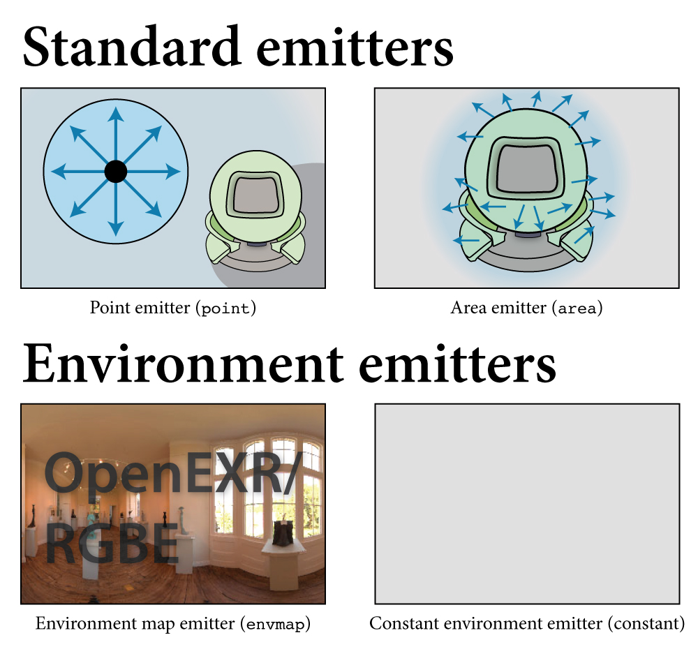
Schematic overview of the emitters in Mitsuba 2. The arrows indicate the directional distribution of light.

Mitsuba 2 supports a number of different emitters/light sources, which can be classified into two main categories: emitters which are located somewhere within the scene, and emitters that surround the scene to simulate a distant environment.

Generally, light sources are specified as children of the <scene> element; for instance, the following snippet instantiates a point light emitter that illuminates a sphere:

<scene version="2.0.0">
    <emitter type="point">
        <spectrum name="intensity" value="1"/>
        <point name="position" x="0" y="0" z="-2"/>
    </emitter>

    <shape type="sphere"/>
</scene>

An exception to this are area lights, which turn a geometric object into a light source. These are specified as children of the corresponding <shape> element:

<scene version="2.0.0">
    <shape type="sphere">
        <emitter type="area">
            <spectrum name="radiance" value="1"/>
        </emitter>
    </shape>
</scene>

Area light (area)

Parameter	Type	Description
radiance	spectrum	Specifies the emitted radiance in units of power per unit area per unit steradian.

This plugin implements an area light, i.e. a light source that emits diffuse illumination from the exterior of an arbitrary shape. Since the emission profile of an area light is completely diffuse, it has the same apparent brightness regardless of the observer’s viewing direction. Furthermore, since it occupies a nonzero amount of space, an area light generally causes scene objects to cast soft shadows.

To create an area light source, simply instantiate the desired emitter shape and specify an area instance as its child:

<shape type="sphere">
    <emitter type="area">
        <spectrum name="radiance" value="1.0"/>
    </emitter>
</shape>

Point light source (point)

Parameter	Type	Description
intensity	spectrum	Specifies the radiant intensity in units of power per unit steradian.
position	point	Alternative parameter for specifying the light source position. Note that only one of the parameters to_world and position can be used at a time.
to_world	transform	Specifies an optional emitter-to-world transformation. (Default: none, i.e. emitter space = world space)

This emitter plugin implements a simple point light source, which uniformly radiates illumination into all directions.

Constant environment emitter (constant)

Parameter	Type	Description
radiance	spectrum	Specifies the emitted radiance in units of power per unit area per unit steradian.

This plugin implements a constant environment emitter, which surrounds the scene and radiates diffuse illumination towards it. This is often a good default light source when the goal is to visualize some loaded geometry that uses basic (e.g. diffuse) materials.

Environment emitter (envmap)

Parameter	Type	Description
filename	string	Filename of the radiance-valued input image to be loaded; must be in latitude-longitude format.
scale	float	A scale factor that is applied to the radiance values stored in the input image. (Default: 1.0)
to_world	transform	Specifies an optional emitter-to-world transformation. (Default: none, i.e. emitter space = world space)

This plugin provides a HDRI (high dynamic range imaging) environment map, which is a type of light source that is well-suited for representing “natural” illumination.

The implementation loads a captured illumination environment from a image in latitude-longitude format and turns it into an infinitely distant emitter. The conventions of this mapping are shown in this image:

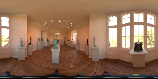
The museum environment map by Bernhard Vogl that is used in many example renderings in this documentation.

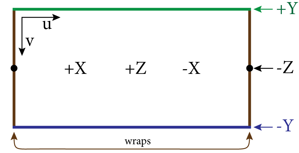
Coordinate conventions used when mapping the input image onto the sphere.

The plugin can work with all types of images that are natively supported by Mitsuba (i.e. JPEG, PNG, OpenEXR, RGBE, TGA, and BMP). In practice, a good environment map will contain high-dynamic range data that can only be represented using the OpenEXR or RGBE file formats. High quality free light probes are available on Paul Debevec’s and Bernhard Vogl’s websites.

Spot light source (spot)

Parameter	Type	Description
intensity	spectrum	Specifies the maximum radiant intensity at the center in units of power per unit steradian. (Default: 1). This cannot be spatially varying (e.g. have bitmap as type).
cutoff_angle	float	Cutoff angle, beyond which the spot light is completely black (Default: 20 degrees)
beam_width	float	Subtended angle of the central beam portion (Default: \(cutoff_angle \times 3/4\))
texture	texture	An optional texture to be projected along the spot light. This must be spatially varying (e.g. have bitmap as type).
to_world	transform	Specifies an optional emitter-to-world transformation. (Default: none, i.e. emitter space = world space)

This plugin provides a spot light with a linear falloff. In its local coordinate system, the spot light is positioned at the origin and points along the positive Z direction. It can be conveniently reoriented using the lookat tag, e.g.:

<emitter type="spot">
    <transform name="to_world">
        <!-- Orient the light so that points from (1, 1, 1) towards (1, 2, 1) -->
        <lookat origin="1, 1, 1" target="1, 2, 1"/>
    </transform>
</emitter>

The intensity linearly ramps up from cutoff_angle to beam_width (both specified in degrees), after which it remains at the maximum value. A projection texture may optionally be supplied.

Two spot lights with different colors and no texture specified.

A spot light with a texture specified.

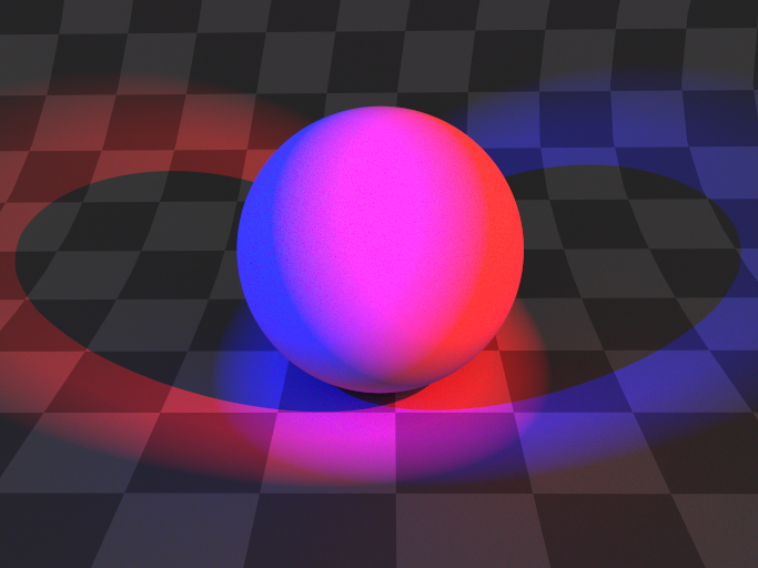
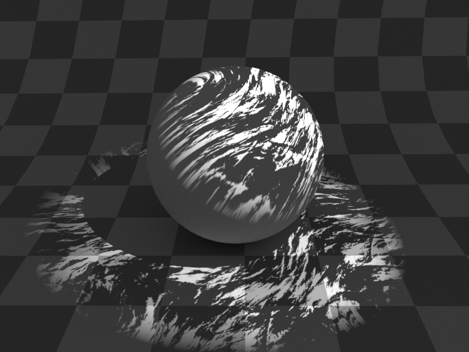
Projection light source (projector)

Parameter	Type	Description
irradiance	texture	2D texture specifying irradiance on the emitter’s virtual image plane, which lies at a distance of \(z=1\) from the pinhole. Note that this does not directly correspond to emitted radiance due to the presence of an additional directionally varying scale factor equal to to the inverse sensitivity profile (a.k.a. importance) of a perspective camera. This ensures that a projection of a constant texture onto a plane is truly constant.
scale	float	A scale factor that is applied to the radiance values stored in the above parameter. (Default: 1.0)
to_world	transform	Specifies an optional camera-to-world transformation. (Default: none (i.e. camera space = world space))
fov	float	Denotes the camera’s field of view in degrees—must be between 0 and 180, excluding the extremes. Alternatively, it is also possible to specify a field of view using the focal_length parameter.
focal_length	string	Denotes the camera’s focal length specified using 35mm film equivalent units. Alternatively, it is also possible to specify a field of view using the fov parameter. See the main description for further details. (Default: 50mm)
fov_axis	string	When the parameter fov is given (and only then), this parameter further specifies the image axis, to which it applies. x: fov maps to the x-axis in screen space. y: fov maps to the y-axis in screen space. diagonal: fov maps to the screen diagonal. smaller: fov maps to the smaller dimension (e.g. x when width < height) larger: fov maps to the larger dimension (e.g. y when width < height) The default is x.

This emitter is the reciprocal counterpart of the perspective camera implemented by the perspective plugin. It accepts exactly the same parameters and employs the same pixel-to-direction mapping. In contrast to the perspective camera, it takes an extra texture (typically of type bitmap) as input that it then projects into the scene, with an optional scaling factor.

Pixels are importance sampled according to their density, hence this operation remains efficient even if only a single pixel is turned on.

A projector lights with constant irradiance (no texture specified).

A projector light with a texture specified.

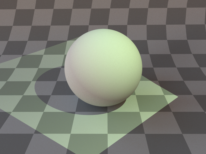
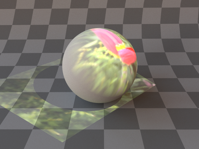
Distant directional emitter (directional)

Parameter	Type	Description
irradiance	spectrum	Spectral irradiance, which corresponds to the amount of spectral power per unit area received by a hypothetical surface normal to the specified direction.
to_world	transform	Emitter-to-world transformation matrix.
direction	vector	Alternative (and exclusive) to to_world. Direction towards which the emitter is radiating in world coordinates.

This emitter plugin implements a distant directional source which radiates a specified power per unit area along a fixed direction. By default, the emitter radiates in the direction of the positive Z axis, i.e. \((0, 0, 1)\).

Sensors

In Mitsuba 2, sensors, along with a film, are responsible for recording radiance measurements in some usable format.

In the XML scene description language, a sensor declaration looks as follows:

<scene version=2.0.0>
    <!-- .. scene contents .. -->

    <sensor type=".. sensor type ..">
        <!-- .. sensor parameters .. -->

        <sampler type=".. sampler type ..">
            <!-- .. sampler parameters .. -->
        </samplers>

        <film type=".. film type ..">
            <!-- .. film parameters .. -->
        </film>
    </sensor>
</scene>

In other words, the sensor declaration is a child element of the <scene> (the particular position in the scene file does not play a role). Nested within the sensor declaration is a sampler instance (see Samplers) and a film instance (see Films).

Sensors in Mitsuba 2 are right-handed. Any number of rotations and translations can be applied to them without changing this property. By default, they are located at the origin and oriented in such a way that in the rendered image, \(+X\) points left, \(+Y\) points upwards, and \(+Z\) points along the viewing direction. Left-handed sensors are also supported. To switch the handedness, flip any one of the axes, e.g. by passing a scale transform like <scale x="-1"/> to the sensor’s to_world parameter.

Perspective pinhole camera (perspective)

Parameter	Type	Description
to_world	transform	Specifies an optional camera-to-world transformation. (Default: none (i.e. camera space = world space))
fov	float	Denotes the camera’s field of view in degrees—must be between 0 and 180, excluding the extremes. Alternatively, it is also possible to specify a field of view using the focal_length parameter.
focal_length	string	Denotes the camera’s focal length specified using 35mm film equivalent units. Alternatively, it is also possible to specify a field of view using the fov parameter. See the main description for further details. (Default: 50mm)
fov_axis	string	When the parameter fov is given (and only then), this parameter further specifies the image axis, to which it applies. x: fov maps to the x-axis in screen space. y: fov maps to the y-axis in screen space. diagonal: fov maps to the screen diagonal. smaller: fov maps to the smaller dimension (e.g. x when width < height) larger: fov maps to the larger dimension (e.g. y when width < height) The default is x.
near_clip, far_clip	float	Distance to the near/far clip planes. (Default: near_clip=1e-2 (i.e. 0.01) and far_clip=1e4 (i.e. 10000))
principal_point_offset_x, principal_point_offset_y	float	Specifies the position of the camera’s principal point relative to the center of the film.
srf	spectrum	If set, sensor response function used to sample wavelengths from. This parameter is ignored if used with nonspectral variants.

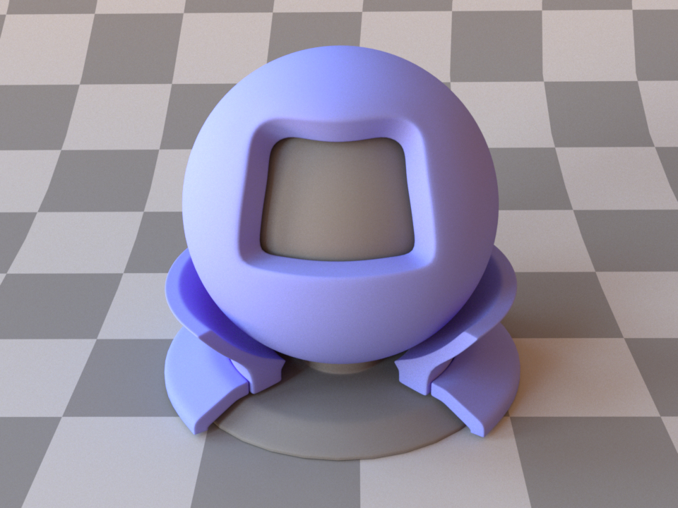
The material test ball viewed through a perspective pinhole camera. (fov=28)

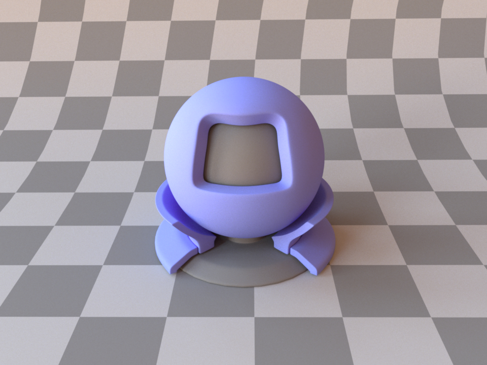
The material test ball viewed through a perspective pinhole camera. (fov=40)

This plugin implements a simple idealized perspective camera model, which has an infinitely small aperture. This creates an infinite depth of field, i.e. no optical blurring occurs.

By default, the camera’s field of view is specified using a 35mm film equivalent focal length, which is first converted into a diagonal field of view and subsequently applied to the camera. This assumes that the film’s aspect ratio matches that of 35mm film (1.5:1), though the parameter still behaves intuitively when this is not the case. Alternatively, it is also possible to specify a field of view in degrees along a given axis (see the fov and fov_axis parameters).

The exact camera position and orientation is most easily expressed using the lookat tag, i.e.:

<sensor type="perspective">
    <transform name="to_world">
        <!-- Move and rotate the camera so that looks from (1, 1, 1) to (1, 2, 1)
            and the direction (0, 0, 1) points "up" in the output image -->
        <lookat origin="1, 1, 1" target="1, 2, 1" up="0, 0, 1"/>
    </transform>
</sensor>

Perspective camera with a thin lens (thinlens)

Parameter	Type	Description
to_world	transform	Specifies an optional camera-to-world transformation. (Default: none (i.e. camera space = world space))
aperture_radius	float	Denotes the radius of the camera’s aperture in scene units.
focus_distance	float	Denotes the world-space distance from the camera’s aperture to the focal plane. (Default: 0)
focal_length	string	Denotes the camera’s focal length specified using 35mm film equivalent units. See the main description for further details. (Default: 50mm)
fov	float	An alternative to focal_length: denotes the camera’s field of view in degrees—must be between 0 and 180, excluding the extremes.
fov_axis	string	When the parameter fov is given (and only then), this parameter further specifies the image axis, to which it applies. x: fov maps to the x-axis in screen space. y: fov maps to the y-axis in screen space. diagonal: fov maps to the screen diagonal. smaller: fov maps to the smaller dimension (e.g. x when width < height) larger: fov maps to the larger dimension (e.g. y when width < height) The default is x.
near_clip, far_clip	float	Distance to the near/far clip planes. (Default: near_clip=1e-2 (i.e. 0.01) and far_clip=1e4 (i.e. 10000))
srf	spectrum	If set, sensor response function used to sample wavelengths from. This parameter is ignored if used with nonspectral variants.

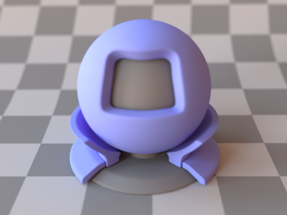
The material test ball viewed through a perspective thin lens camera. (aperture_radius=0.1)

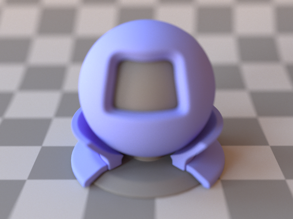
The material test ball viewed through a perspective thin lens camera. (aperture_radius=0.2)

This plugin implements a simple perspective camera model with a thin lens at its circular aperture. It is very similar to the perspective plugin except that the extra lens element permits rendering with a specifiable (i.e. non-infinite) depth of field. To configure this, it has two extra parameters named aperture_radius and focus_distance.

By default, the camera’s field of view is specified using a 35mm film equivalent focal length, which is first converted into a diagonal field of view and subsequently applied to the camera. This assumes that the film’s aspect ratio matches that of 35mm film (1.5:1), though the parameter still behaves intuitively when this is not the case. Alternatively, it is also possible to specify a field of view in degrees along a given axis (see the fov and fov_axis parameters).

The exact camera position and orientation is most easily expressed using the lookat tag, i.e.:

<sensor type="thinlens">
    <transform name="to_world">
        <!-- Move and rotate the camera so that looks from (1, 1, 1) to (1, 2, 1)
            and the direction (0, 0, 1) points "up" in the output image -->
        <lookat origin="1, 1, 1" target="1, 2, 1" up="0, 0, 1"/>
    </transform>

    <!-- Focus on the target -->
    <float name="focus_distance" value="1"/>
    <float name="aperture_radius" value="0.1"/>
</sensor>

Multi distant radiance meter (mdistant)

Parameter	Type	Description
directions	string	Comma-separated list of directions in which the sensors are pointing in world coordinates.
target	point or nested shape plugin	Optional. Define the ray target sampling strategy. If this parameter is unset, ray target points are sampled uniformly on the cross section of the scene’s bounding sphere. If a point is passed, rays will target it. If a shape plugin is passed, ray target points will be sampled from its surface.

This sensor plugin aggregates an arbitrary number of distant directional sensors which records the spectral radiance leaving the scene in specified directions. It is the aggregation of multiple distant sensors.

By default, ray target points are sampled from the cross section of the scene’s bounding sphere. The target parameter can be set to restrict ray target sampling to a specific subregion of the scene. The recorded radiance is averaged over the targeted geometry.

Ray origins are positioned outside of the scene’s geometry.

Warning

If this sensor is used with a targeting strategy leading to rays not hitting the scene’s geometry (e.g. default targeting strategy), it will pick up ambient emitter radiance samples (or zero values if no ambient emitter is defined). Therefore, it is almost always preferrable to use a nondefault targeting strategy.

Important

This sensor must be used with a film with size (N, 1), where N is the number of aggregated sensors, and is best used with a default box reconstruction filter.

Irradiance meter (irradiancemeter)

Parameter	Type	Description
srf	spectrum	If set, sensor response function used to sample wavelengths from. This parameter is ignored if used with nonspectral variants.

This sensor plugin implements an irradiance meter, which measures the incident power per unit area over a shape which it is attached to. This sensor is used with films of 1 by 1 pixels.

If the irradiance meter is attached to a mesh-type shape, it will measure the irradiance over all triangles in the mesh.

This sensor is not instantiated on its own but must be defined as a child object to a shape in a scene. To create an irradiance meter, simply instantiate the desired sensor shape and specify an irradiancemeter instance as its child:

<shape type="sphere">
    <sensor type="irradiancemeter">
        <!-- film -->
    </sensor>
</shape>

Distant directional sensor (distant)

Parameter	Type	Description
to_world	transform	Sensor-to-world transformation matrix.
direction	vector	Alternative (and exclusive) to to_world. Direction orienting the sensor’s reference hemisphere.
orientation	vector	If direction is set, this vector parameter can be used to control film orientation. The orientation is given by the projection of orientation onto the plane of normal direction, and the up vector defined as \(\mathrm{up} = \mathrm{direction} \times \mathrm{orientation}\). If direction is unset, this parameter has no effect.
flip_directions	boolean	If true, flip the directions of sampled rays. Default: false
ray_target	point or nested shape plugin	Optional. Define the ray target sampling strategy. If this parameter is unset, ray target points are sampled uniformly on the cross section of the scene’s bounding sphere. If a point is passed, rays will target it. If a shape plugin is passed, ray target points will be sampled from its surface.
ray_origin	nested shape plugin	Optional. Specify the ray origin computation strategy. If this parameter is unset, ray origins will be positioned using the bounding sphere of the scene so as to ensure that they lie outside of any geometry. If a shape plugin is passed, ray origin points will be positioned by projecting the sampled target point onto the shape following the sampled ray direction. If the projection is impossible, an invalid ray is returned with zero weights. Note: ray invalidation occurs per-lane in packet modes.

This sensor plugin implements a distant directional sensor which records radiation leaving the scene in a given direction. It records the spectral radiance leaving the scene in the specified direction. Rays target points are sampled from the cross section of the scene’s bounding sphere and their origins are positioned outside of the scene’s geometry.

Based on the film size, the ray direction sampling strategy will vary:

• if a 1x1 film is passed, rays directions will be equal to -direction (unless flip_directions is true, in which case they will be equal to direction);

• if a Nx1 film is passed (i.e. if film height is reduced to 1), ray directions will be sampled from the intersection of the hemisphere defined by -direction and the (vector) plane generated by orientation and direction;

• if a NxM film is passed, ray directions will be sampled in the hemisphere defined by -direction.

Rays sampled from this sensor can be tuned so as to target a specific region of the scene using the ray_target parameter. The recorded radiance is averaged over the targeted geometry.

The positioning of the origin of those rays can also be controlled using the ray_origin. This is particularly useful when the scene has a dimension much smaller than the others and it is not necessary that ray origins are located at the scene’s bounding sphere.

Warning

If this sensor is used with a targeting strategy leading to rays not hitting the scene’s geometry (e.g. default targeting strategy), it will pick up ambiant emitter radiance samples (or zero values if no ambiant emitter is defined). Therefore, it is almost always preferrable to use a nondefault targeting strategy.

Radiance meter (radiancemeter)

Parameter	Type	Description
to_world	transform	Specifies an optional camera-to-world transformation. (Default: none (i.e. camera space = world space))
origin	point	Location from which the sensor will be recording in world coordinates. Must be used with origin.
direction	vector	Alternative (and exclusive) to to_world. Direction in which the sensor is pointing in world coordinates. Must be used with origin.
srf	spectrum	If set, sensor response function used to sample wavelengths from. This parameter is ignored if used with nonspectral variants.

This sensor plugin implements a simple radiance meter, which measures the incident power per unit area per unit solid angle along a certain ray. It can be thought of as the limit of a standard perspective camera as its field of view tends to zero. This sensor is used with films of 1 by 1 pixels.

Such a sensor is useful for conducting virtual experiments and testing the renderer for correctness.

By default, the sensor is located at the origin and performs a measurement in the positive Z direction (0,0,1). This can be changed by providing a custom to_world transformation, or a pair of origin and direction values. If both types of transformation are specified, the to_world transformation has higher priority.

Distant fluxmeter sensor (distantflux)

Parameter	Type	Description
to_world	transform	Sensor-to-world transformation matrix.
target	point or nested shape plugin	Optional. Define the ray target sampling strategy. If this parameter is unset, ray target points are sampled uniformly on the cross section of the scene’s bounding sphere. If a point is passed, rays will target it. If a shape plugin is passed, ray target points will be sampled from its surface.
origin	nested shape plugin	Optional. Specify the ray origin computation strategy. If this parameter is unset, ray origins will be positioned using the bounding sphere of the scene so as to ensure that they lie outside of any geometry. If a shape plugin is passed, ray origin points will be positioned by projecting the sampled target point onto the shape following the sampled ray direction. If the projection is impossible, an invalid ray is returned with zero weights. Note: ray invalidation occurs per-lane in packet modes.

This sensor plugin implements a distant sensor which records the radiative flux density leaving the scene (in W/m², scaled by scene unit length). It covers a hemisphere defined by its to_world parameter and mapped to film coordinates.

The to_world transform is best set using a look_at(). The default orientation covers a hemisphere defined by the [0, 0, 1] direction, and the up film direction is set to [0, 1, 0].

Using a 1x1 film with a stratified sampler is recommended. A different film size can also be used. In that case, the exitant flux is given by the sum of all pixel values.

By default, ray target points are sampled from the cross section of the scene’s bounding sphere. The target parameter can be set to restrict ray target sampling to a specific subregion of the scene. The recorded radiance is averaged over the targeted geometry.

Ray origins are positioned outside of the scene’s geometry.

Warning

If this sensor is used with a targeting strategy leading to rays not hitting the scene’s geometry (e.g. default targeting strategy), it will pick up ambient emitter radiance samples (or zero values if no ambient emitter is defined). Therefore, it is almost always preferrable to use a nondefault targeting strategy.

Multi radiance meter (mradiancemeter)

Parameter	Type	Description
origins	string	Comma separated list of locations from which the sensors will be recording in world coordinates.
directions	string	Comma separated list of directions in which the sensors are pointing in world coordinates.

This sensor plugin aggregates multiple radiance meters. It makes it possible to benefit from film-based parallelization when using radiance meters, which is not possible with the radiancemeter plugin due to its film size of 1x1.

The origin points and direction vectors for this sensor are specified as a list of floating point values, where three subsequent values will be grouped into a point or vector respectively.

The following snippet shows how to specify a mradiancemeter with two sensors, one located at (1, 0, 0) and pointing in the direction (-1, 0, 0), the other located at (0, 1, 0) and pointing in the direction (0, -1, 0).

<sensor version="2.0.0" type="mradiancemeter">
    <string name="origins" value="1, 0, 0, 0, 1, 0"/>
    <string name="directions" value="-1, 0, 0, 0, -1, 0"/>
    <film type="hdrfilm">
        <integer name="width" value="2"/>
        <integer name="height" value="1"/>
        <rfilter type="box"/>
    </film>
</sensor>

<shape type="sphere">
    <sensor type="irradiancemeter">
        <!-- film -->
    </sensor>
</shape>

Textures

The following section describes the available texture data sources. In Mitsuba 2, textures are objects that can be attached to certain surface scattering model parameters to introduce spatial variation. In the documentation, these are listed as supporting the texture type. See the last sections about BSDFs for many examples.

Textures take an (optional) <transform> called to_uv which can be used to translate, scale, or rotate the lookup into the texture accordingly.

An example in XML looks the following:

<scene version=2.0.0>
    <!-- Create a BSDF that supports textured parameters -->
    <bsdf type=".. BSDF type .." id="my_textured_material">
        <texture type=".. texture type .." name=".. parameter name ..">
            <!-- .. Texture parameters go here .. -->

            <transform name="to_uv">
                <!-- Scale texture by factor of 2 -->
                <scale x="2" y="2"/>
                <!-- Offset texture by [0.5, 1.0] -->
                <translate x="0.5" y="1.0"/>
            </transform>
        </texture>

        <!-- .. Non-spatially varying BSDF parameters ..-->
    </bsdf>
</scene>

Similar to BSDFs, named textures can alternatively defined at the top level of the scene and later referenced. This is particularly useful if the same texture would be loaded many times otherwise.

<scene version=2.0.0>
    <!-- Create a named texture at the top level -->
    <texture type=".. texture type .." id="my_named_texture">
        <!-- .. Texture parameters go here .. -->

        <transform name="to_uv">
            <!-- .. Transform parameters .. -->
        </transform>
    </texture>

    <!-- Create a BSDF that supports textured parameters -->
    <bsdf type=".. BSDF type ..">
        <!-- Example of referencing a named texture -->
        <ref id="my_named_texture" name=".. parameter name .."/>

        <!-- .. Non-spatially varying BSDF parameters ..-->
    </bsdf>
</scene>

Bitmap texture (bitmap)

Parameter	Type	Description
filename	string	Filename of the bitmap to be loaded
filter_type	string	Specifies how pixel values are interpolated and filtered when queried over larger UV regions. The following options are currently available: bilinear (default): perform bilinear interpolation, but no filtering. nearest: disable filtering and interpolation. In this mode, the plugin performs nearest neighbor lookups of texture values.
wrap_mode	string	Controls the behavior of texture evaluations that fall outside of the \([0, 1]\) range. The following options are currently available: repeat (default): tile the texture infinitely. mirror: mirror the texture along its boundaries. clamp: clamp coordinates to the edge of the texture.
raw	boolean	Should the transformation to the stored color data (e.g. sRGB to linear, spectral upsampling) be disabled? You will want to enable this when working with bitmaps storing normal maps that use a linear encoding. (Default: false)
to_uv	transform	Specifies an optional 3x3 transformation matrix that will be applied to UV values. A 4x4 matrix can also be provided, in which case the extra row and column are ignored.

This plugin provides a bitmap texture that performs interpolated lookups given a JPEG, PNG, OpenEXR, RGBE, TGA, or BMP input file.

When loading the plugin, the data is first converted into a usable color representation for the renderer:

• In rgb modes, sRGB textures are converted into a linear color space.

• In spectral modes, sRGB textures are spectrally upsampled to plausible smooth spectra [JH19] and stored an intermediate representation that enables efficient queries at render time.

• In monochrome modes, sRGB textures are converted to grayscale.

These conversions can alternatively be disabled with the raw flag, e.g. when textured data is already in linear space or does not represent colors at all.

Checkerboard texture (checkerboard)

Parameter	Type	Description
color0, color1	spectrum or texture	Color values for the two differently-colored patches (Default: 0.4 and 0.2)
to_uv	transform	Specifies an optional 3x3 UV transformation matrix. A 4x4 matrix can also be provided. In that case, the last row and columns will be ignored. (Default: none)

This plugin provides a simple procedural checkerboard texture with customizable colors.

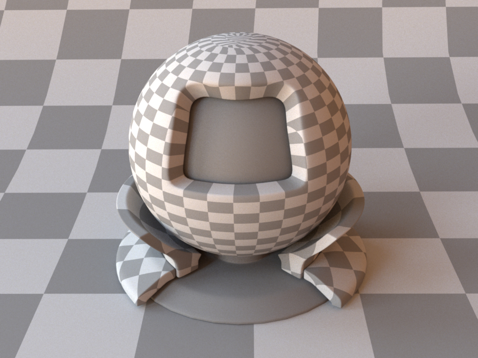
Checkerboard applied to the material test object as well as the ground plane.

Spectral grid (gridvolume_spectral)

This plugin implements a gridded volume data source using an arbitrary regular spectrum. It should be preferred over the gridvolume plugin when proper spectral data is to be used.

In practice, this plugin can be seen as a combination of the gridvolume and regular plugins. Evaluations outside of the covered spectral range will return 0.

WARNING: This plugin is currently in alpha stage and can be subject to deep changes.

Parameter	Type	Description
filename	string	Filename of the volume data file to be loaded
use_grid_bbox	boolean	If True, use the bounding box information contained in the loaded file. (Default: False)
wrap_mode	string	Controls the behavior of texture evaluations that fall outside of the [0,1] range. The following options are currently available: - repeat: tile the texture infinitely - mirror: mirror the texture along its boundaries - clamp (default): clamp coordinates to the edge of the texture
lambda_min	float	Lower bound of the covered spectral interval
lambda_max	float	Upper bound of the covered spectral interval

Mesh attribute texture (mesh_attribute)

Parameter	Type	Description
name	string	Name of the attribute to evaluate. It should always start with "vertex_" or "face_".
scale	float	Scaling factor applied to the interpolated attribute value during evalutation. (Default: 1.0)

This plugin provides a simple mechanism to expose Mesh attributes (e.g. vertex color) as a texture.

Bunny with random vertex color (using barycentric interpolation).

Bunny with random face color.

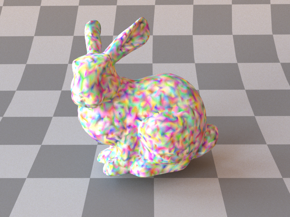
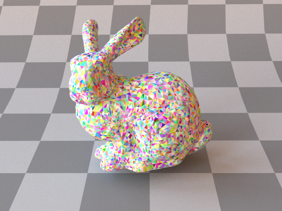
The following XML snippet describes a mesh with diffuse material, whose reflectance is specified using the vertex_color attribute of that mesh:

<shape type="ply">
    <string name="filename" value="my_mesh_with_vertex_color_attr.ply"/>

    <bsdf type="diffuse">
        <texture type="mesh_attribute" name="reflectance">
            <string name="name" value="vertex_color"/>
        </texture>
    </bsdf>
</shape>

Note

For spectral variants of the renderer (e.g. scalar_spectral), when a mesh attribute name contains the string "color", the tri-stimulus RGB values will be converted to rgb2spec model coefficients automatically.

Spectra

This section describes the plugins behind spectral reflectance or emission used in Mitsuba 2. On an implementation level, these behave very similarly to the texture plugins described earlier (but lacking their spatially varying property) and can thus be used similarly as either BSDF or emitter parameters:

<scene version=2.0.0>
    <bsdf type=".. BSDF type ..">
        <!-- Explicitly add a uniform spectrum plugin -->
        <spectrum type=".. spectrum type .." name=".. parameter name ..">
            <!-- Spectrum parameters go here -->
        </spectrum>
    </bsdf>
</scene>

In practice, it is however discouraged to instantiate plugins in this explicit way and the XML scene description parser directly parses a number of common (shorter) <spectrum> and <rgb> tags See the corresponding section about the scene file format for details.

The following two tables summarize which underlying plugins get instantiated in each case, accounting for differences between reflectance and emission properties and all different color modes. Each plugin is briefly summarized below.

XML description	Monochrome mode	RGB mode	Spectral mode
<spectrum name=".." value="0.5"/>	uniform	uniform	uniform
<spectrum name=".." value="400:0.1, 700:0.2"/>	uniform	srgb	regular/irregular
<spectrum name=".." filename=".."/>	uniform	srgb	regular/irregular
<rgb name=".." value="0.5, 0.2, 0.5"/>	srgb	srgb	srgb

Spectra used for reflectance (within BSDFs)

XML description	Monochrome mode	RGB mode	Spectral mode
<spectrum name=".." value="0.5"/>	uniform	uniform	d65
<spectrum name=".." value="400:0.1, 700:0.2"/>	uniform	srgb_d65	regular/irregular
<spectrum name=".." filename=".."/>	uniform	srgb_d65	regular/irregular
<rgb name=".." value="0.5, 0.2, 0.5"/>	srgb_d65	srgb_d65	srgb_d65

Spectra used for emission (within emitters)

Uniform spectrum (uniform)

In its default form, this spectrum returns a constant reflectance or emission value between 360 and 830nm. When using spectral variants, the covered spectral interval can be specified tuned using its full XML specification; the plugin will return 0 outside of the covered spectral range.

Parameter	Type	Description
value	float	Returned value
lambda_min	float	Lower bound of the covered spectral interval. (Default: MTS_WAVELENGTH_MIN)
lambda_max	float	Upper bound of the covered spectral interval. (Default: MTS_WAVELENGTH_MAX)

Regular spectrum (regular)

This spectrum returns linearly interpolated reflectance or emission values from regularly placed samples.

Irregular spectrum (irregular)

This spectrum returns linearly interpolated reflectance or emission values from irregularly placed samples.

sRGB spectrum (srgb)

In spectral render modes, this smooth spectrum is the result of the spectral upsampling process [JH19] used by the system. In RGB render modes, this spectrum represents a constant RGB value. In monochrome modes, this spectrum represents a constant luminance value.

D65 spectrum (d65)

The CIE Standard Illuminant D65 corresponds roughly to the average midday light in Europe, also called a daylight illuminant. It is the default emission spectrum used for light sources in all spectral rendering modes.

sRGB D65 spectrum (srgb_d65)

This is a convenience wrapper around both the srgb and d65 plugins and returns their product. This is the current default behavior in spectral rendering modes for light sources specified from an RGB color value.

Blackbody spectrum (blackbody)

This is a black body radiation spectrum for a specified temperature And therefore takes a single float-valued parameter temperature (in Kelvins).

This is the only spectrum type that needs to be explicitly instantiated in its full XML description:

<shape type=".. shape type ..">
    <emitter type="area">
        <spectrum type="blackbody" name="radiance">
            <float name="temperature" value="5000"/>
        </spectrum>
    </emitter>
</shape>

This spectrum type only makes sense for specifying emission and is unavailable in non-spectral rendering modes.

Note that attaching a black body spectrum to the intensity property of a emitter introduces physical units into the rendering process of Mitsuba 2, which is ordinarily a unitless system. Specifically, the black body spectrum has units of power (\(W\)) per unit area (\(m^{-2}\)) per steradian (\(sr^{-1}\)) per unit wavelength (\(nm^{-1}\)). As a consequence, your scene should be modeled in meters for this plugin to work properly.

Discrete spectrum (discrete)

Parameter	Type	Description
wavelengths	string	A comma-separated list of wavelengths to sample.
values	string	A comma-separated list of spectrum values associated with each wavelength. Alternatively, a single value can be passed and used for all wavelengths. (Default: “1”)
pmf	string	A comma-separated list of probability mass density associated with each wavelength. If unspecified, all wavelengths are equiprobable.

This spectrum can only be used through its full XML specification.

This spectrum plugin samples wavelengths from a discrete distribution. Consequently, it will always return 0 when queried for evaluation or PDF values.

Black body radiance spectrum (blackbody_interpolated)

Parameter	Type	Description
temperature	float	Black body temperature (in K).

This plugin computes the spectral radiance (in W/m²/sr/nm) in emitted by a black body at the specified temperature (in K).

This implementation relies on a piecewise-linear discretisation in a dimensionless wavelength space to mitigate the effects temperature can have on the spectral profile’s curvature.

Integrators

In Mitsuba 2, the different rendering techniques are collectively referred to as integrators, since they perform integration over a high-dimensional space. Each integrator represents a specific approach for solving the light transport equation—usually favored in certain scenarios, but at the same time affected by its own set of intrinsic limitations. Therefore, it is important to carefully select an integrator based on user-specified accuracy requirements and properties of the scene to be rendered.

In the XML description language, a single integrator is usually instantiated by declaring it at the top level within the scene, e.g.

<scene version=2.0.0>
    <!-- Instantiate a unidirectional path tracer,
         which renders paths up to a depth of 5 -->
    <integrator type="path">
        <integer name="max_depth" value="5"/>
    </integrator>

    <!-- Some geometry to be rendered -->
    <shape type="sphere">
        <bsdf type="diffuse"/>
    </shape>
</scene>

This section gives an overview of the available choices along with their parameters.

Almost all integrators use the concept of path depth. Here, a path refers to a chain of scattering events that starts at the light source and ends at the camera. It is oten useful to limit the path depth when rendering scenes for preview purposes, since this reduces the amount of computation that is necessary per pixel. Furthermore, such renderings usually converge faster and therefore need fewer samples per pixel. Then reference-quality is desired, one should always leave the path depth unlimited.

The Cornell box renderings below demonstrate the visual effect of a maximum path depth. As the paths are allowed to grow longer, the color saturation increases due to multiple scattering interactions with the colored surfaces. At the same time, the computation time increases.

max. depth = 1

max. depth = 2

max. depth = 3

max. depth = \(\infty\)

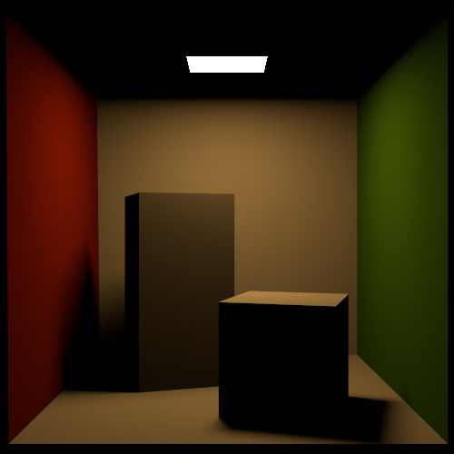
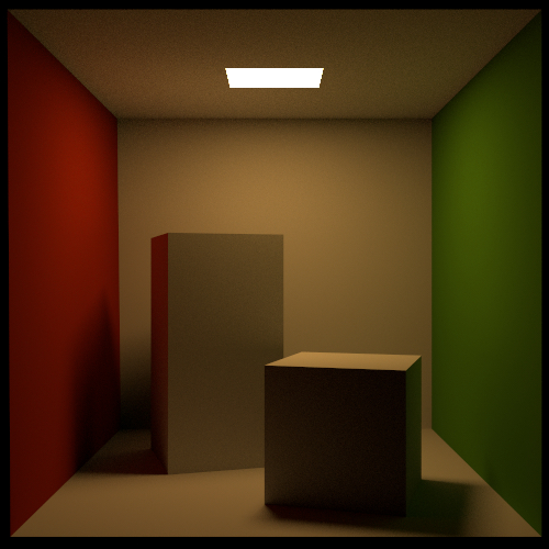
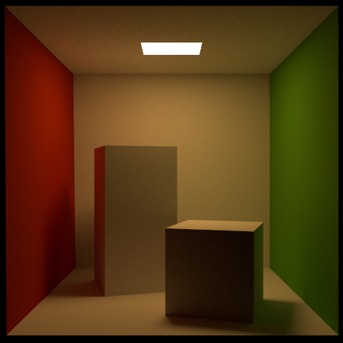
Mitsuba counts depths starting at 1, which corresponds to visible light sources (i.e. a path that starts at the light source and ends at the camera without any scattering interaction in between.) A depth-2 path (also known as “direct illumination”) includes a single scattering event like shown here:

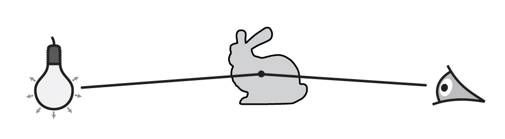
Direct illumination integrator (direct)

Parameter	Type	Description
shading_samples	integer	This convenience parameter can be used to set both emitter_samples and bsdf_samples at the same time.
emitter_samples	integer	Optional more fine-grained parameter: specifies the number of samples that should be generated using the direct illumination strategies implemented by the scene’s emitters. (Default: set to the value of shading_samples)
bsdf_samples	integer	Optional more fine-grained parameter: specifies the number of samples that should be generated using the BSDF sampling strategies implemented by the scene’s surfaces. (Default: set to the value of shading_samples)
hide_emitters	boolean	Hide directly visible emitters. (Default: no, i.e. false)

(a) BSDF sampling only

(b) Emitter sampling only

(c) MIS between both sampling strategies

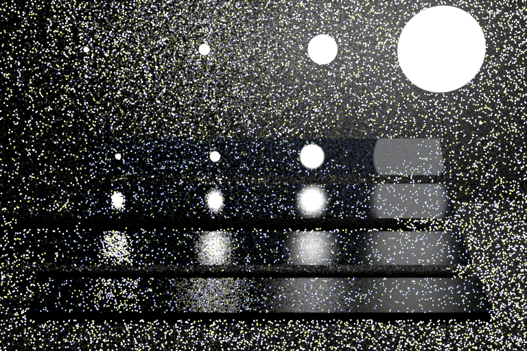
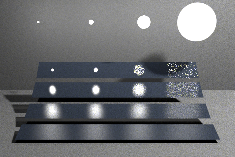
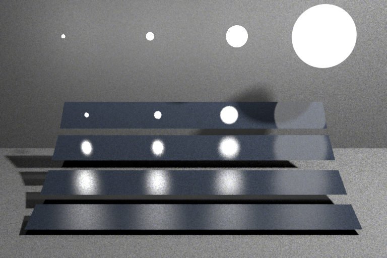
This integrator implements a direct illumination technique that makes use of multiple importance sampling: for each pixel sample, the integrator generates a user-specifiable number of BSDF and emitter samples and combines them using the power heuristic. Usually, the BSDF sampling technique works very well on glossy objects but does badly everywhere else (a), while the opposite is true for the emitter sampling technique (b). By combining these approaches, one can obtain a rendering technique that works well in both cases (c).

The number of samples spent on either technique is configurable, hence it is also possible to turn this plugin into an emitter sampling-only or BSDF sampling-only integrator.

Note

This integrator does not handle participating media or indirect illumination.

Path tracer (path)

Parameter	Type	Description
max_depth	integer	Specifies the longest path depth in the generated output image (where -1 corresponds to \(\infty\)). A value of 1 will only render directly visible light sources. 2 will lead to single-bounce (direct-only) illumination, and so on. (Default: -1)
rr_depth	integer	Specifies the minimum path depth, after which the implementation will start to use the russian roulette path termination criterion. (Default: 5)
hide_emitters	boolean	Hide directly visible emitters. (Default: no, i.e. false)

This integrator implements a basic path tracer and is a good default choice when there is no strong reason to prefer another method.

To use the path tracer appropriately, it is instructive to know roughly how it works: its main operation is to trace many light paths using random walks starting from the sensor. A single random walk is shown below, which entails casting a ray associated with a pixel in the output image and searching for the first visible intersection. A new direction is then chosen at the intersection, and the ray-casting step repeats over and over again (until one of several stopping criteria applies).

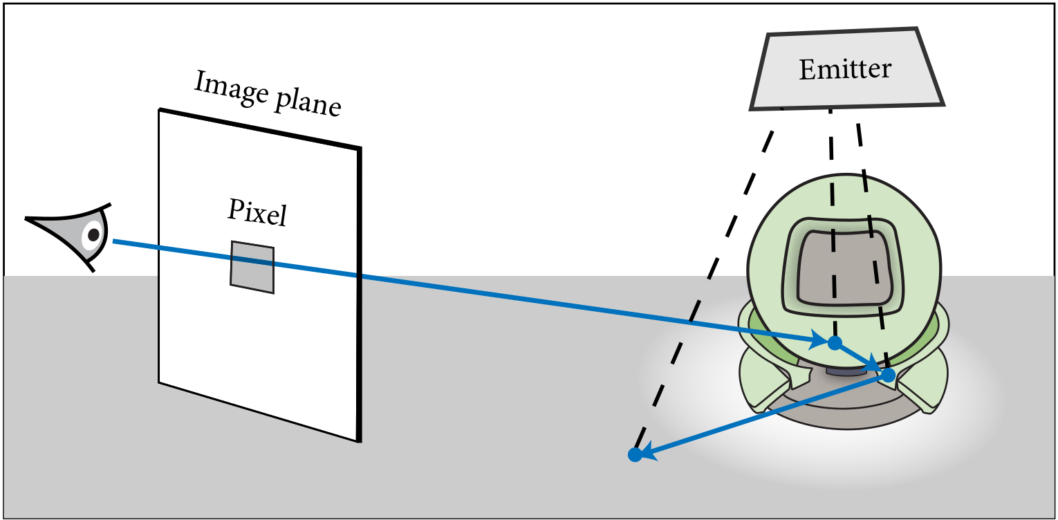
At every intersection, the path tracer tries to create a connection to the light source in an attempt to find a complete path along which light can flow from the emitter to the sensor. This of course only works when there is no occluding object between the intersection and the emitter.

This directly translates into a category of scenes where a path tracer can be expected to produce reasonable results: this is the case when the emitters are easily “accessible” by the contents of the scene. For instance, an interior scene that is lit by an area light will be considerably harder to render when this area light is inside a glass enclosure (which effectively counts as an occluder).

Like the direct plugin, the path tracer internally relies on multiple importance sampling to combine BSDF and emitter samples. The main difference in comparison to the former plugin is that it considers light paths of arbitrary length to compute both direct and indirect illumination.

Note

This integrator does not handle participating media

Arbitrary Output Variables integrator (aov)

Parameter	Type	Description
aovs	string	List of <name>:<type> pairs denoting the enabled AOVs.
(Nested plugin)	integrator	Sub-integrators (can have more than one) which will be sampled along the AOV integrator. Their respective output will be put into distinct images.

This integrator returns one or more AOVs (Arbitrary Output Variables) describing the visible surfaces.

Scene rendered with a path tracer

Depth AOV

Normal AOV

Position AOV

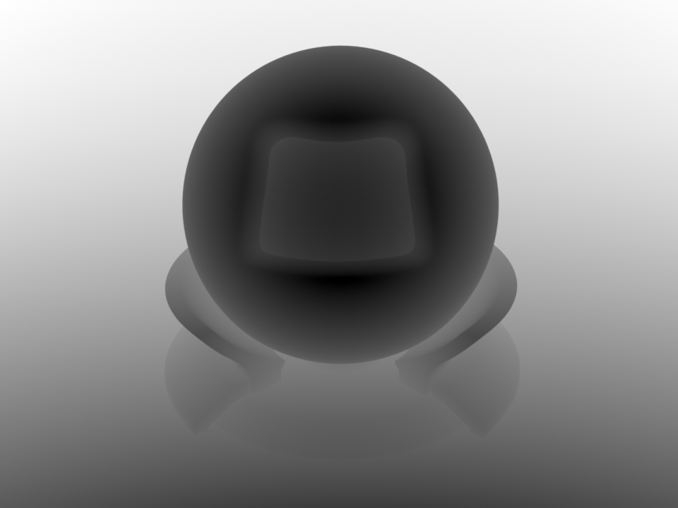
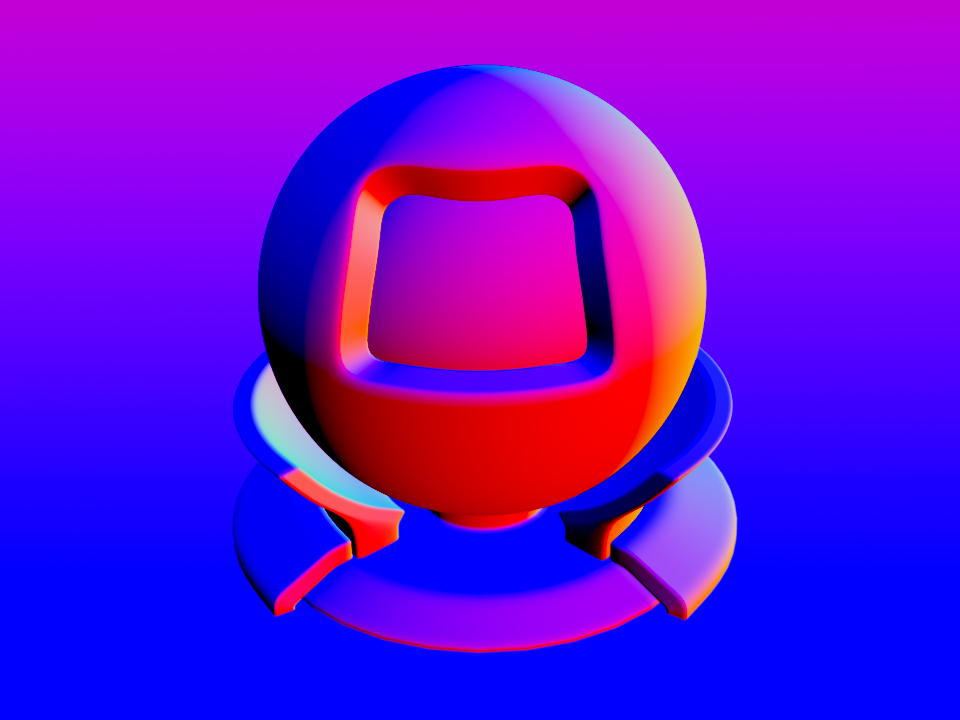
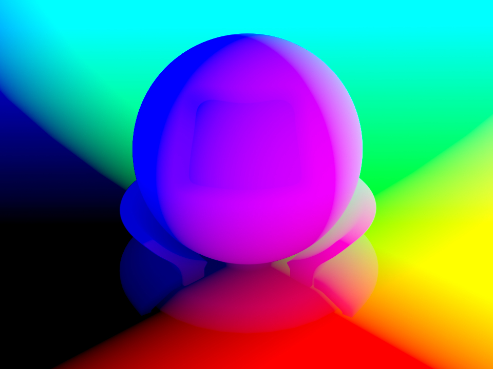
Here is an example on how to enable the depth and shading normal AOVs while still rendering the image with a path tracer. The RGBA image produces by the path tracer will be stored in the [my_image.R, my_image.G, my_image.B, my_image.A] channels of the EXR output file.

<integrator type="aov">
    <string name="aovs" value="dd.y:depth,nn:sh_normal"/>
    <integrator type="path" name="my_image"/>
</integrator>

Currently, the following AOVs types are available:

• depth: Distance from the pinhole.

• position: World space position value.

• uv: UV coordinates.

• geo_normal: Geometric normal.

• sh_normal: Shading normal.

• dp_du, dp_dv: Position partials wrt. the UV parameterization.

• duv_dx, duv_dy: UV partials wrt. changes in screen-space.

Moment integrator (moment)

Parameter	Type	Description
(Nested plugin)	integrator	Sub-integrators (can have more than one) which will be sampled along the AOV integrator. Their respective XYZ output will be put into distinct images.

This integrator returns one AOVs recording the second moment of the samples of the nested integrator.

Narrow bins integrator (nbins)

Parameter	Type	Description
wavelengths	string	A comma-separated list of wavelengths used for bin detection.
tolerance	float	Tolerance for bin detection (in nm), i.e. narrow bin width. (Default: 1e-5)
(Nested plugin)	integrator	Sub-integrator (only one can be specified) which will be sampled along the narrow bins integrator.

This integrator computes radiance for selected wavelengths in spectral mode. It is intended to be used when wavelengths are sampled from discrete spectral distributions.

In practice, it accumulates contributions in very narrow spectral bins whose width is controlled by the tolerance parameter. In addition to accumulated contributions for each wavelength, the integrator records the number of contributions for each wavelength, which should be used during a post-processing step to normalize the obtained values.

Note

This integrator can only be used with non-polarized spectral variants.

Warning

If used improperly, this integrator is very likely to yield meaningless results!

Stokes vector integrator (stokes)

Parameter	Type	Description
(Nested plugin)	integrator	Sub-integrator (only one can be specified) which will be sampled along the Stokes integrator. In polarized rendering modes, its output Stokes vector is written into distinct images.

This integrator returns a multi-channel image describing the complete measured polarization state at the sensor, represented as a Stokes vector \(\mathbf{s}\).

Here we show an example monochrome output in a scene with two dielectric and one conductive sphere that all affect the polarization state of the (initially unpolarized) light.

The first entry corresponds to usual radiance, whereas the remaining three entries describe the polarization of light shown as false color images (green: positive, red: negative).

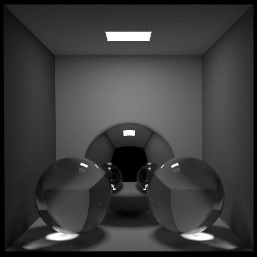
“\(\mathbf{s}_0\)”: radiance

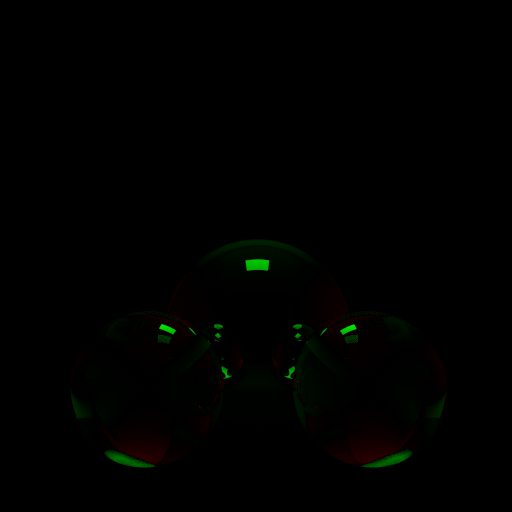
“\(\mathbf{s}_1\)”: horizontal vs. vertical polarization

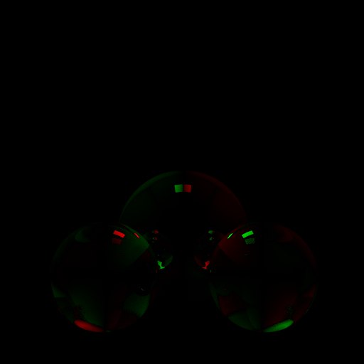
“\(\mathbf{s}_2\)”: positive vs. negative diagonal polarization

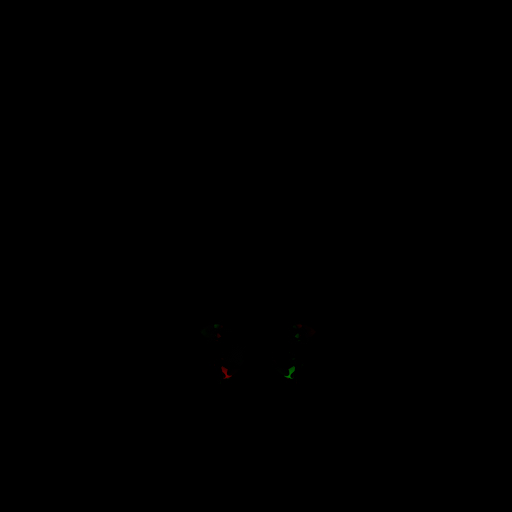
“\(\mathbf{s}_3\)”: right vs. left circular polarization

In the following example, a normal path tracer is nested inside the Stokes vector integrator:

<integrator type="stokes">
    <integrator type="path">
        <!-- path tracer parameters -->
    </integrator>
</integrator>

Volumetric path tracer with null scattering (volpath)

Todo

Not documented yet.

Samplers

When rendering an image, Mitsuba 2 has to solve a high-dimensional integration problem that involves the geometry, materials, lights, and sensors that make up the scene. Because of the mathematical complexity of these integrals, it is generally impossible to solve them analytically — instead, they are solved numerically by evaluating the function to be integrated at a large number of different positions referred to as samples. Sample generators are an essential ingredient to this process: they produce points in a (hypothetical) infinite dimensional hypercube \([0, 1]^{\infty}\) that constitute the canonical representation of these samples.

To do its work, a rendering algorithm, or integrator, will send many queries to the sample generator. Generally, it will request subsequent 1D or 2D components of this infinite-dimensional point and map them into a more convenient space (for instance, positions on surfaces). This allows it to construct light paths to eventually evaluate the flow of light through the scene.

Independent sampler (independent)

Parameter	Type	Description
sample_count	integer	Number of samples per pixel (Default: 4)
seed	integer	Seed offset (Default: 0)

The independent sampler produces a stream of independent and uniformly distributed pseudorandom numbers. Internally, it relies on the PCG32 random number generator by Melissa O’Neill.

This is the most basic sample generator; because no precautions are taken to avoid sample clumping, images produced using this plugin will usually take longer to converge. Looking at the figures below where samples are projected onto a 2D unit square, we see that there are both regions that don’t receive many samples (i.e. we don’t know much about the behavior of the function there), and regions where many samples are very close together (which likely have very similar values), which will result in higher variance in the rendered image.

This sampler is initialized using a deterministic procedure, which means that subsequent runs of Mitsuba should create the same image. In practice, when rendering with multiple threads and/or machines, this is not true anymore, since the ordering of samples is influenced by the operating system scheduler. Although these should be absolutely negligible, with relative errors on the order of the machine epsilon (\(6\cdot 10^{-8}\)) in single precision.

1024 samples projected onto the first two dimensions.

64 samples projected onto the first two dimensions and their projection on both 1D axis (top and right plot).

Stratified sampler (stratified)

Parameter	Type	Description
sample_count	integer	Number of samples per pixel. This number should be a square number (Default: 4)
seed	integer	Seed offset (Default: 0)
jitter	boolean	Adds additional random jitter withing the stratum (Default: True)

The stratified sample generator divides the domain into a discrete number of strata and produces a sample within each one of them. This generally leads to less sample clumping when compared to the independent sampler, as well as better convergence.

Independent sampler - 16 samples per pixel

Stratified sampler - 16 samples per pixel

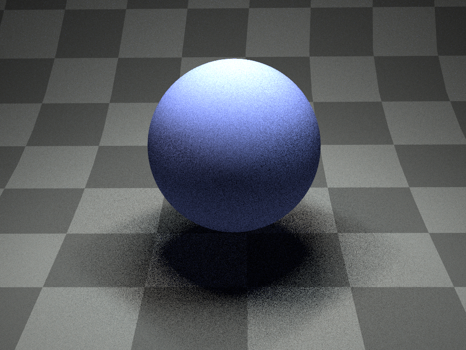
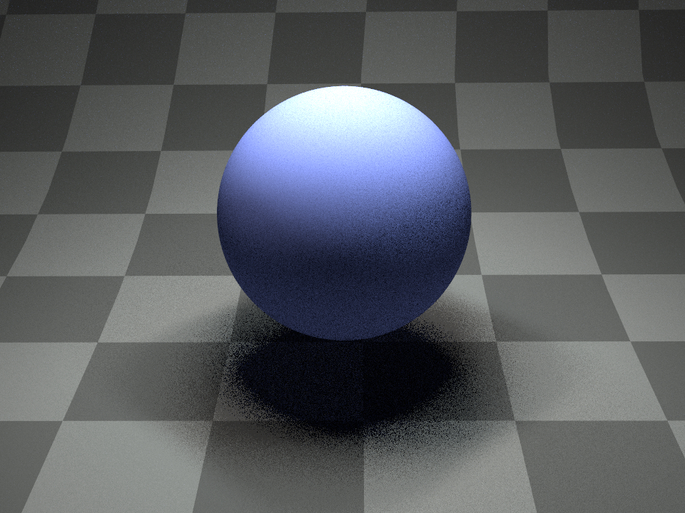
1024 samples projected onto the first two dimensions which are well distributed if we compare to the independent sampler.

64 samples projected in 2D and on both 1D axis (top and right plot). Every strata contains a single sample creating a good distribution when projected in 2D. Projections on both 1D axis still exhibit sample clumping which will result in higher variance, for instance when sampling a thin streched rectangular area light.

Correlated Multi-Jittered sampler (multijitter)

Parameter	Type	Description
sample_count	integer	Number of samples per pixel. The sampler may internally choose to slightly increase this value to create a subdivision into strata that has an aspect ratio close to one. (Default: 4)
seed	integer	Seed offset (Default: 0)
jitter	boolean	Adds additional random jitter withing the substratum (Default: True)

This plugin implements the methods introduced in Pixar’s tech memo [Ken67].

Unlike the previously described stratified sampler, multi-jittered sample patterns produce samples that are well stratified in 2D but also well stratified when projected onto one dimension. This can greatly reduce the variance of a Monte-Carlo estimator when the function to evaluate exhibits more variation along one axis of the sampling domain than the other.

This sampler achieves this by first placing samples in a canonical arrangement that is stratified in both 2D and 1D. It then shuffles the x-coordinate of the samples in every columns and the y-coordinate in every rows. Fortunately, this process doesn’t break the 2D and 1D stratification. Kensler’s method futher reduces sample clumpiness by correlating the shuffling applied to the columns and the rows.

Independent sampler - 16 samples per pixel

Correlated Multi-Jittered sampler - 16 samples per pixel

1024 samples projected onto the first two dimensions.

64 samples projected onto the first two dimensions and their projection on both 1D axis (top and right plot). As expected, the samples are well stratified both in 2D and 1D.

Orthogonal Array sampler (orthogonal)

Parameter	Type	Description
sample_count	integer	Number of samples per pixel. This value has to be the square of a prime number. (Default: 4)
strength	integer	Orthogonal array’s strength (Default: 2)
seed	integer	Seed offset (Default: 0)
jitter	boolean	Adds additional random jitter withing the substratum (Default: True)

This plugin implements the Orthogonal Array sampler generator introduced by Jarosz et al. [JEK+19]. It generalizes correlated multi-jittered sampling to higher dimensions by using orthogonal arrays (OAs). An OA of strength \(s\) has the property that projecting the generated samples to any combination of \(s\) dimensions will always result in a well stratified pattern. In other words, when \(s=2\) (default value), the high-dimentional samples are simultaneously stratified in all 2D projections as if they had been produced by correlated multi-jittered sampling. By construction, samples produced by this generator are also well stratified when projected on both 1D axis.

This sampler supports OA of strength other than 2, although this isn’t recommended as the stratification of 2D projections of those samples wouldn’t be ensured anymore.

Independent sampler - 25 samples per pixel

Orthogonal Array sampler - 25 samples per pixel

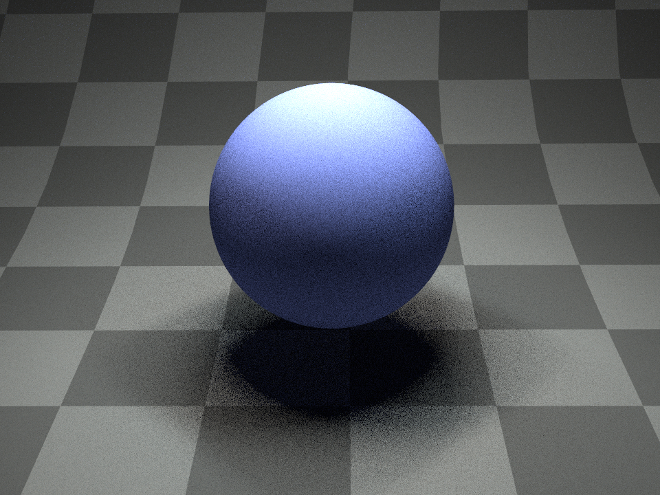
1369 samples projected onto the first two dimensions.

49 samples projected onto the first two dimensions and their projection on both 1D axis (top and right plot). The pattern is well stratified in both 2D and 1D projections. This is true for every pair of dimensions of the high-dimentional samples.

Low discrepancy sampler (ldsampler)

This plugin implements a simple hybrid sampler that combines aspects of a Quasi-Monte Carlo sequence with a pseudorandom number generator based on a technique proposed by Kollig and Keller [KK02]. It is a good and fast general-purpose sample generator. Other QMC samplers exist that can generate even better distributed samples, but this comes at a higher cost in terms of performance. This plugin is based on Mitsuba 1’s default sampler (also called ldsampler).

Roughly, the idea of this sampler is that all of the individual 2D sample dimensions are first filled using the same (0, 2)-sequence, which is then randomly scrambled and permuted using a shuffle network. The name of this plugin stems from the fact that, by construction, (0, 2)-sequences achieve a low star discrepancy, which is a quality criterion on their spatial distribution.

Independent sampler - 16 samples per pixel

Low-discrepancy sampler - 16 samples per pixel

1024 samples projected onto the first two dimensions.

A projection of the first 64 samples onto the first two dimensions and their projection on both 1D axis (top and right plot). The 1D stratification is perfect as this sampler doesn’t add additional random perturbation to the sample positions.

1024 samples projected onto the 32th and 33th dimensions, which look almost identical. However, note that the points have been scrambled to reduce correlations between dimensions.

A projection of the first 64 samples onto the 32th and 33th dimensions.

Films

A film defines how conducted measurements are stored and converted into the final output file that is written to disk at the end of the rendering process.

In the XML scene description language, a normal film configuration might look as follows:

<scene version=2.0.0>
    <!-- .. scene contents -->

    <sensor type=".. sensor type ..">
        <!-- .. sensor parameters .. -->

        <!-- Write to a high dynamic range EXR image -->
        <film type="hdrfilm">
            <!-- Specify the desired resolution (e.g. full HD) -->
            <integer name="width" value="1920"/>
            <integer name="height" value="1080"/>

            <!-- Use a Gaussian reconstruction filter. For details
                 on these, refor to the next subsection -->
            <rfilter type="gaussian"/>
        </film>
    </sensor>
</scene>

The <film> plugin should be instantiated nested inside a <sensor> declaration. Note how the output filename is never specified—it is automatically inferred from the scene filename and can be manually overridden by passing the configuration parameter -o to the mitsuba executable when rendering from the command line.

High dynamic range film (hdrfilm)

Parameter	Type	Description
width, height	integer	Width and height of the camera sensor in pixels Default: 768, 576)
file_format	string	Denotes the desired output file format. The options are openexr (for ILM’s OpenEXR format), rgbe (for Greg Ward’s RGBE format), or pfm (for the Portable Float Map format). (Default: openexr)
pixel_format	string	Specifies the desired pixel format of output images. The options are luminance, luminance_alpha, rgb, rgba, xyz and xyza. (Default: rgba)
component_format	string	Specifies the desired floating point component format of output images. The options are float16, float32, or uint32. (Default: float16)
crop_offset_y, crop_offset_y, crop_width, crop_height	integer	These parameters can optionally be provided to select a sub-rectangle of the output. In this case, only the requested regions will be rendered. (Default: Unused)
high_quality_edges	boolean	If set to true, regions slightly outside of the film plane will also be sampled. This may improve the image quality at the edges, especially when using very large reconstruction filters. In general, this is not needed though. (Default: false, i.e. disabled)
(Nested plugin)	rfilter	Reconstruction filter that should be used by the film. (Default: gaussian, a windowed Gaussian filter)

This is the default film plugin that is used when none is explicitly specified. It stores the captured image as a high dynamic range OpenEXR file and tries to preserve the rendering as much as possible by not performing any kind of post processing, such as gamma correction—the output file will record linear radiance values.

When writing OpenEXR files, the film will either produce a luminance, luminance/alpha, RGB(A), or XYZ(A) tristimulus bitmap having a float16, float32, or uint32-based internal representation based on the chosen parameters. The default configuration is RGBA with a float16 component format, which is appropriate for most purposes.

For OpenEXR files, Mitsuba 2 also supports fully general multi-channel output; refer to the aov or stokes plugins for details on how this works.

The plugin can also write RLE-compressed files in the Radiance RGBE format pioneered by Greg Ward (set file_format=rgbe), as well as the Portable Float Map format (set file_format=pfm). In the former case, the component_format and pixel_format parameters are ignored, and the output is float8-compressed RGB data. PFM output is restricted to float32-valued images using the rgb or luminance pixel formats. Due to the superior accuracy and adoption of OpenEXR, the use of these two alternative formats is discouraged however.

When RGB(A) output is selected, the measured spectral power distributions are converted to linear RGB based on the CIE 1931 XYZ color matching curves and the ITU-R Rec. BT.709-3 primaries with a D65 white point.

The following XML snippet discribes a film that writes a full-HD RGBA OpenEXR file:

<film type="hdrfilm">
    <string name="pixel_format" value="rgba"/>
    <integer name="width" value="1920"/>
    <integer name="height" value="1080"/>
</film>

Reconstruction filters

Image reconstruction filters are responsible for converting a series of radiance samples generated jointly by the sampler and integrator into the final output image that will be written to disk at the end of a rendering process. This section gives a brief overview of the reconstruction filters that are available in Mitsuba. There is no universally superior filter, and the final choice depends on a trade-off between sharpness, ringing, and aliasing, and computational efficiency.

Desireable properties of a reconstruction filter are that it sharply captures all of the details that are displayable at the requested image resolution, while avoiding aliasing and ringing. Aliasing is the incorrect leakage of high-frequency into low-frequency detail, and ringing denotes oscillation artifacts near discontinuities, such as a light-shadow transiton.

Box filter (box)

This is the fastest, but also about the worst possible reconstruction filter, since it is prone to severe aliasing. It is included mainly for completeness, though some rare situations may warrant its use.

Tent filter (tent)

Simple tent (triangular) filter. This reconstruction filter never suffers from ringing and usually causes less aliasing than a naive box filter. When rendering scenes with sharp brightness discontinuities, this may be useful; otherwise, negative-lobed filters may be preferable (e.g. Mitchell-Netravali or Lanczos Sinc).

Gaussian filter (gaussian)

This is a windowed Gaussian filter with configurable standard deviation. It often produces pleasing results, and never suffers from ringing, but may occasionally introduce too much blurring.

When no reconstruction filter is explicitly requested, this is the default choice in Mitsuba.

Takes a standard deviation parameter (stddev) which is set to 0.5 pixels be default.

Mitchell filter (mitchell)

Separable cubic spline reconstruction filter by Mitchell and Netravali [MN88]. This is often a good compromise between sharpness and ringing.

This plugin has two float-valued parameters B and C that correspond to the two parameters in the original paper. By default, these are set to the recommended value of \(1/3\), but can be tweaked if desired.

Catmull-Rom filter (catmullrom)

Special version of the Mitchell-Netravali filter with constants B and C configured to match the Catmull-Rom spline. It usually does a better job at at preserving sharp features at the cost of more ringing.

Lanczos filter (lanczos)

This is a windowed version of the theoretically optimal low-pass filter. It is generally one of the best available filters in terms of producing sharp high-quality output. Its main disadvantage is that it produces strong ringing around discontinuities, which can become a serious problem when rendering bright objects with sharp edges (a directly visible light source will for instance have black fringing artifacts around it). This is also the computationally slowest reconstruction filter.

This plugin has an integer-valued parameter named lobes, that sets the desired number of filter side-lobes. The higher, the closer the filter will approximate an optimal low-pass filter, but this also increases ringing. Values of 2 or 3 are common (3 is the default).