More advanced examples¶

Differentiating textures¶

The previous example demonstrated differentiation of a scalar color parameter. We will now show how to work with textured parameters, focusing on the example of an environment map emitter.

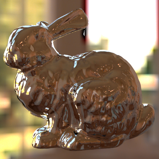
../../_images/bunny.jpg — A metallic Stanford bunny surrounded by an environment map.¶

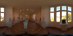
../../_images/museum.jpg — The ground-truth environment map that we will attempt to recover from the image on the left.¶

The example scene can be downloaded here and contains a metallic Stanford bunny surrounded by a museum-like environment. As before, we load the scene and enumerate its differentiable parameters:

import enoki as ek
import mitsuba
mitsuba.set_variant('gpu_autodiff_rgb')

from mitsuba.core import Float, Thread
from mitsuba.core.xml import load_file
from mitsuba.python.util import traverse
from mitsuba.python.autodiff import render, write_bitmap, Adam

# Load example scene
Thread.thread().file_resolver().append('bunny')
scene = load_file('bunny/bunny.xml')

# Find differentiable scene parameters
params = traverse(scene)

We then make a backup copy of the ground-truth environment map and generate a reference rendering

# Make a backup copy
param_res = params['my_envmap.resolution']
param_ref = Float(params['my_envmap.data'])

# Discard all parameters except for one we want to differentiate
params.keep(['my_envmap.data'])

# Render a reference image (no derivatives used yet)
image_ref = render(scene, spp=16)
crop_size = scene.sensors()[0].film().crop_size()
write_bitmap('out_ref.png', image_ref, crop_size)

Let’s now change the environment map into a uniform white lighting environment. The my_envmap.data parameter is a RGBA bitmap linearized into a 1D array of size param_res[0] x param_res[1] x 4 (125’000).

# Change to a uniform white lighting environment
params['my_envmap.data'] = ek.full(Float, 1.0, len(param_ref))
params.update()

Finally, we jointly estimate all 125K parameters using gradient-based optimization. The optimization loop is identical to previous examples except that we can now also write out the current environment image in each iteration.

# Construct an Adam optimizer that will adjust the parameters 'params'
opt = Adam(params, lr=.02)

for it in range(100):
    # Perform a differentiable rendering of the scene
    image = render(scene, optimizer=opt, unbiased=True, spp=1)
    write_bitmap('out_%03i.png' % it, image, crop_size)
    write_bitmap('envmap_%03i.png' % it, params['my_envmap.data'],
                 (param_res[0], param_res[1]))

    # Objective: MSE between 'image' and 'image_ref'
    ob_val = ek.hsum(ek.sqr(image - image_ref)) / len(image)

    # Back-propagate errors to input parameters
    ek.backward(ob_val)

    # Optimizer: take a gradient step
    opt.step()

    # Compare iterate against ground-truth value
    err_ref = ek.hsum(ek.sqr(param_ref - params['my_envmap.data']))
    print('Iteration %03i: error=%g' % (it, err_ref[0]))

The following video shows the convergence behavior during the first 100 iterations. The image rapidly resolves to the target image. The small black regions in the image correspond to parts of the mesh where inter-reflection was ignored due to a limit on the maximum number of light bounces.

The following image shows the reconstructed environment map at each step. Unobserved regions are unaffected by gradient steps and remain white.

This image is still fairly noisy and even contains some negative (!) regions. This is because the optimization problem defined above is highly ambiguous due to the loss of information that occurs in the forward rendering model above. The solution we found optimizes the objective well (i.e. the rendered image matches the target), but the reconstructed texture may not match our expectation. In such a case, it may be advisable to introduce further regularization (non-negativity, smoothness, etc.).

Table Of Contents

More advanced examples¶

Differentiating textures¶