Differentiable rendering

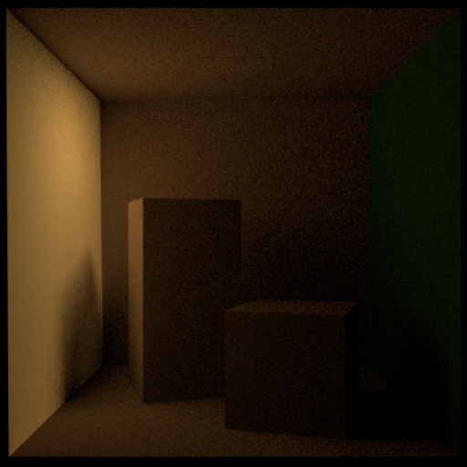
We now progressively build up a simple example application that showcases differentiation and optimization of a light transport simulation involving the well-known Cornell Box scene that can be downloaded here.

Please make the following three changes to the cbox.xml file:

1. ldsampler must be replaced by independent (ldsampler has not yet been ported to Mitsuba 2). Note that the sample count specified here will be overriden in the optimization script below.

2. The integrator at the top should be defined as follows:

   <integrator type="path">
       <integer name="max_depth" value="3"/>
   </integrator>
   

3. The film should specify a box reconstruction filter instead of gaussian.

   <rfilter type="box"/>
   

In the context of differentiable rendering, we are typically interested in rendering many fairly low-quality images as quickly as possible, and the above changes reduce the quality of the rendered images accordingly.

Enumerating scene parameters

Since differentiable rendering requires a starting guess (i.e. an initial scene configuration), most applications will begin by loading the Cornell box scene and enumerating and selecting scene parameters that will subsequently be differentiated:

import enoki as ek
import mitsuba
mitsuba.set_variant('gpu_autodiff_rgb')

from mitsuba.core import Thread
from mitsuba.core.xml import load_file
from mitsuba.python.util import traverse

# Load the Cornell Box
Thread.thread().file_resolver().append('cbox')
scene = load_file('cbox/cbox.xml')

# Find differentiable scene parameters
params = traverse(scene)
print(params)

The call to traverse() in the second-to-last line serves this purpose. It returns a dictionary-like mitsuba.python.util.ParameterMap instance, which exposes modifiable and differentiable scene parameters. Passing it to print() yields the following summary (abbreviated):

ParameterMap[
    ...
  * box.reflectance.value,
  * white.reflectance.value,
  * red.reflectance.value,
  * green.reflectance.value,
  * light.reflectance.value,
    ...
  * OBJMesh.emitter.radiance.value,
    OBJMesh.vertex_count,
    OBJMesh.face_count,
    OBJMesh.faces,
  * OBJMesh.vertex_positions,
  * OBJMesh.vertex_normals,
  * OBJMesh.vertex_texcoords,
    OBJMesh_1.vertex_count,
    OBJMesh_1.face_count,

    OBJMesh_1.faces,
  * OBJMesh_1.vertex_positions,
  * OBJMesh_1.vertex_normals,
  * OBJMesh_1.vertex_texcoords,
    ...
]

The Cornell box scene consists of a single light source, and multiple multiple meshes and BRDFs. Each component contributes certain entries to the above list—for instance, meshes specify their face and vertex counts in addition to per-face (.faces) and per-vertex data (.vertex_positions, .vertex_normals, .vertex_texcoords). Each BRDF adds a .reflectance.value entry. Not all of these parameters are differentiable—some, e.g., store integer values. The asterisk (*) on the left of some parameters indicates that they are differentiable.

The parameter names are generated using a simple naming scheme based on the position in the scene graph and class name of the underlying implementation. Whenever an object was assigned a unique identifier via the id="..." attribute in the XML scene description, this identifier has precedence. For instance, The red.reflectance.value entry corresponds to the albedo of the following declaration in the original scene description:

<bsdf type="diffuse" id="red">
    <spectrum name="reflectance" value="400:0.04, 404:0.046, ..., 696:0.635, 700:0.642"/>
</bsdf>

We can also query the ParameterMap to see the actual parameter value:

print(params['red.reflectance.value'])

# Prints:
# [[0.569717, 0.0430141, 0.0443234]]

Here, we can see how Mitsuba converted the original spectral curve from the above XML fragment into an RGB value due to the gpu_autodiff_rgb variant being used to run this example.

In most cases, we will only be interested in differentiating a small subset of the (typically very large) parameter map. Use the ParameterMap.keep() method to discard all entries except for the specified list of keys.

params.keep(['red.reflectance.value'])
print(params)

# Prints:
# ParameterMap[
#   * red.reflectance.value
# ]

Let’s also make a backup copy of this color value for later use.

from mitsuba.core import Color3f
param_ref = Color3f(params['red.reflectance.value'])

Problem statement

In contrast to the previous example on using the Python API to render images, the differentiable rendering path involves another rendering function mitsuba.python.autodiff.render() that is more optimized for this use case. It directly returns a GPU array containing the generated image. The function write_bitmap() reshapes the output into an image of the correct size and exports it to any of the supported image formats (OpenEXR, PNG, JPG, RGBE, PFM) while automatically performing format conversion and gamma correction in the case of an 8-bit output format.

Using this functionality, we will now generate a reference image using 8 samples per pixel (spp).

# Render a reference image (no derivatives used yet)
from mitsuba.python.autodiff import render, write_bitmap
image_ref = render(scene, spp=8)
crop_size = scene.sensors()[0].film().crop_size()
write_bitmap('out_ref.png', image_ref, crop_size)

Our first experiment is going to be very simple: we will change the color of the red wall and then try to recover the original color using differentiation along with the reference image generated above.

For this, let’s first change the current color value: the parameter map enables such changes without having to reload the scene. The call to the ParameterMap.update() method at the end is mandatory to inform changed scene objects that they should refresh their internal state.

# Change the left wall into a bright white surface
params['red.reflectance.value'] = [.9, .9, .9]
params.update()

Gradient-based optimization

Mitsuba can either optimize scene parameters in standalone mode using optimization algorithms implemented on top of Enoki, or it can be used as a differentiable node within a larger PyTorch computation graph. Communication between PyTorch and Enoki causes certain overheads, hence we generally recommend standalone mode unless your computation contains elements where PyTorch provides a clear advantage (for example, neural network building blocks like fully connected layers or convolutions). The remainder of this section discusses standalone mode, and the section on PyTorch integration shows how to adapt the example code for PyTorch.

Mitsuba ships with standard optimizers including Stochastic Gradient Descent (SGD) with and without momentum, as well as Adam [KB14] We will instantiate the latter and optimize our reduced ParameterMap params with a learning rate of 0.2. The optimizer class automatically requests derivative information for selected parameters and updates their value after each step, hence it is not necessary to directly modify params or call ek.set_requires_gradient as explained in the introduction.

# Construct an Adam optimizer that will adjust the parameters 'params'
from mitsuba.python.autodiff import Adam
opt = Adam(params, lr=.2)

The remaining commands are all part of a loop that executes 100 differentiable rendering iterations.

for it in range(100):
    # Perform a differentiable rendering of the scene
    image = render(scene, optimizer=opt, unbiased=True, spp=1)

    write_bitmap('out_%03i.png' % it, image, crop_size)

Note

Regarding bias in gradients: One potential issue when naively differentiating a rendering algorithm is that the same set of Monte Carlo sample is used to generate both the primal output (i.e. the image) along with derivative output. When the rendering algorithm and objective are jointly differentiated, we end up with expectations of products that do not satisfy the equality \(\mathbb{E}[X Y]=\mathbb{E}[X]\, \mathbb{E}[Y]\) due to correlations between \(X\) and \(Y\) that result from this sample re-use.

The unbiased=True parameter to the render() function switches the function into a special unbiased mode that de-correlates primal and derivative components, which boils down to rendering the image twice and naturally comes at some cost in performance \((\sim 1.6 \times\!)\). Often, biased gradients are good enough, in which case unbiased=False should be specified instead.

Note

Regarding the number of samples per pixel: An extremely low number of samples per pixel (spp=1) is being used in the differentiable rendering iterations above, which produces both noisy renderings and noisy gradients. Alternatively, we could have used many more samples to take correspondingly larger gradient steps (i.e. a higher lr=.. parameter to the optimizer). We generally find the first variant with few samples preferable, since it greatly reduces memory usage and is more adaptive to changes in the parameter value.

Still within the for loop, we can now evaluate a suitable objective function, propagate derivatives with respect to the objective, and take gradient steps.

# for loop body (continued)
    # Objective: MSE between 'image' and 'image_ref'
    ob_val = ek.hsum(ek.sqr(image - image_ref)) / len(image)

    # Back-propagate errors to input parameters
    ek.backward(ob_val)

    # Optimizer: take a gradient step
    opt.step()

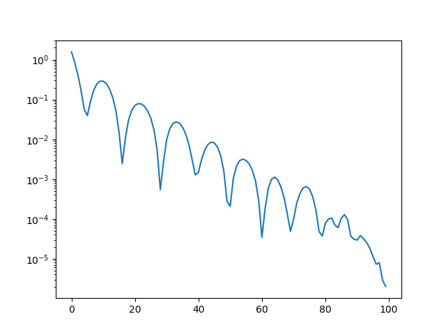
We can also plot the error during each iteration. Note that it makes little sense to visualize the objective ob_val, since differences between image and image_ref are by far dominated by Monte Carlo noise that is not related to the parameter being optimized. Since we know the “true” target parameter in this scene (previously stored in param_ref), we can validate the convergence of the iteration:

err_ref = ek.hsum(ek.sqr(param_ref - params['red.reflectance.value']))
print('Iteration %03i: error=%g' % (it, err_ref[0]))

The following video shows a recording of the convergence during the first 100 iterations. The gradient steps quickly recover the original red color of the left wall.

Note the oscillatory behavior, which is also visible in the convergence plot shown below. This indicates that the learning rate is potentially set to an overly large value.

Note

Regarding performance: this optimization should finish very quickly. On an NVIDIA Titan RTX, it takes roughly 50 ms per iteration when the write_bitmap routine is commented out, and 27 ms per iteration when furthermore setting unbiased=False.

We have noticed that simultaneous GPU usage by another application (e.g. Chrome or Firefox) that appears completely innocuous (YouTube open in a tab, etc.) can reduce differentiable rendering performance ten-fold. If you find that your numbers are very different from the ones mentioned above, try closing all other software.

Note

The full Python script of this tutorial can be found in the file: docs/examples/10_diff_render/invert_cbox.py.

Forward-mode differentiation

The previous example demonstrated reverse-mode differentiation (a.k.a. backpropagation) where a desired small change to the output image was converted into a small change to the scene parameters. Mitsuba and Enoki can also propagate derivatives in the other direction, i.e., from input parameters to the output image. This technique, known as forward mode differentiation, is not usable for optimization, as each parameter must be handled using a separate rendering pass. That said, this mode can be very educational since it enables visualizations of the effect of individual scene parameters on the rendered image.

Forward mode differentiable rendering begins analogously to reverse mode, by declaring parameters and marking them as differentiable (we do so manually instead of using an mitsuba.python.autodiff.Optimizer).

# Keep track of derivatives with respect to one parameter
param_0 = params['red.reflectance.value']
ek.set_requires_gradient(param_0)

# Differentiable simulation
image = render(scene, spp=32)

Once the computation has been recorded, we can specify a perturbation with respect to the previously flagged parameter and forward-propagate it through the graph.

# Assign the gradient [1, 1, 1] to the 'red.reflectance.value' input
ek.set_gradient(param_0, [1, 1, 1], backward=False)

from mitsuba.core import Float

# Forward-propagate previously assigned gradients. The set_gradient call
# above already indicated which derivatives to propagate, hence we use the
# static FloatD.forward() function. See the Enoki documentation for further
# explanations of the various ways in which derivatives can be propagated.
Float.forward()

See Enoki’s documentation regarding automatic differentiation for further details on these steps. Finally, we can write the resulting gradient visualization to disk.

# The gradients have been propagated to the output image
image_grad = ek.gradient(image)

# .. write them to a PNG file
crop_size = scene.sensors()[0].film().crop_size()
write_bitmap('out.png', image_grad, crop_size)

This should produce a result similar to the following image:

Observe how changing the color of the red wall has a global effect on the entire image due to global illumination. Since we are differentiating with respect to albedo, the red color disappears.

Note

The full Python script of this tutorial can be found in the file: docs/examples/10_diff_render/forward_diff.py.