Custom applications

The Python API can also be used to directly interface with lower-level components of the renderer. In this section, we show how to instantiate a rough conductor BSDF and plot its output for some combinations of incident and outgoing directions.

import enoki as ek
import mitsuba

# Set the desired mitsuba variant
mitsuba.set_variant('packet_rgb')

from mitsuba.core import Float, Vector3f
from mitsuba.core.xml import load_string
from mitsuba.render import SurfaceInteraction3f, BSDFContext


def sph_dir(theta, phi):
    """ Map spherical to Euclidean coordinates """
    st, ct = ek.sincos(theta)
    sp, cp = ek.sincos(phi)
    return Vector3f(cp*st, sp*st, ct)


# Load desired BSDF plugin
bsdf = load_string("""<bsdf version='2.0.0' type='roughconductor'>
                          <float name="alpha" value="0.2"/>
                          <string name="distribution" value="ggx"/>
                      </bsdf>""")

# Create a (dummy) surface interaction to use for the evaluation
si = SurfaceInteraction3f()

# Specify an incident direction with 45 degrees elevation
si.wi = sph_dir(ek.pi * 45 / 180, 0.0)

# Create grid in spherical coordinates and map it onto the sphere
res = 300
theta_o, phi_o = ek.meshgrid(
    ek.linspace(Float, 0,     ek.pi,     res),
    ek.linspace(Float, 0, 2 * ek.pi, 2 * res)
)
wo = sph_dir(theta_o, phi_o)

# Evaluate the whole array (18000 directions) at once
values = bsdf.eval(BSDFContext(), si, wo)

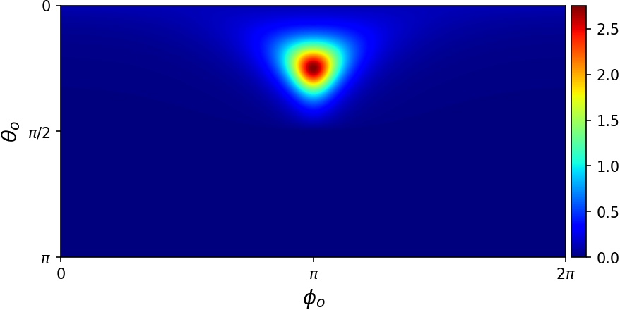
The generated array of values can then be further processed in NumPy or plotted using matplotlib:

import numpy as np
import matplotlib.pyplot as plt
from mpl_toolkits.axes_grid1 import make_axes_locatable

# Extract red channel of BRDF values and reshape into 2D grid
values_r = np.array(values)[:, 0]
values_r = values_r.reshape(2 * res, res).T

# Plot values for spherical coordinates
fig, ax = plt.subplots(figsize=(12, 7))

im = ax.imshow(values_r, extent=[0, 2 * np.pi, np.pi, 0],
               cmap='jet', interpolation='bicubic')

ax.set_xlabel(r'$\phi_o$', size=14)
ax.set_xticks([0, np.pi, 2 * np.pi])
ax.set_xticklabels(['0', '$\\pi$', '$2\\pi$'])
ax.set_ylabel(r'$\theta_o$', size=14)
ax.set_yticks([0, np.pi / 2, np.pi])
ax.set_yticklabels(['0', '$\\pi/2$', '$\\pi$'])

divider = make_axes_locatable(ax)
cax = divider.append_axes("right", size="3%", pad=0.05)
plt.colorbar(im, cax=cax)

# fig.savefig("bsdf_eval.jpg", dpi=150, bbox_inches='tight', pad_inches=0)
plt.show()

This creates the following visualization:

Note

The full Python script of this tutorial can be found in the file: docs/examples/05_bsdf_eval/bsdf_eval.py.